Chapter 5 Phylogenetic Tree Decomposition

There are several aspects of microbiome data that make statistical analysis difficult. Issues include high dimensionality with large numbers of OTUs, sparsity due to small OTU counts, and potential correlations among counts of different OTUs. These aspects can cause problems when attempting to perform inference on the abundances of taxonomic units. Furthermore, simply analyzing regression results one OTU at a time fails to take into account the dependencies across different bacterial populations in the gut.

To address these concerns, we applied a “Phylogenetic Tree Decomposition” to our microbiome data. This methodology replicates concepts introduced in PhyloScan (Tang, Ma, & Nicolae, 2018) and DTM (T. Wang & Zhao, 2017). Using a phylogenetic tree can summarize the evolutionary relationships amongst the OTUs, allowing us to have a better context of their functional relationships and enriching the overall model fitting process.

With our completed filtration of our samples, we constructed a phylogenetic tree to represent the relations between our samples. We used the DECIPHER package in R to first perform multiple-alignment on the sequences in our ASV sequence table (Wright, 2016). We then used the R package “phangorn” to fit a UPGMA tree based upon our sequences (Schliep, 2016).

Our full tree was a binary tree with a single root node. There were a total of 11048 leaf nodes, and 11047 internal nodes. Our filtered ASV table has a total of 462 rows, each corresponding to a distinct sample. Each of the 11048 columns in our ASV table represents a leaf in the phylogenetic tree. With the initial abundances for each sample, we propagated our way up through the phylogenetic tree, determining the counts going left and right at each of our 11047 internal nodes. This process was repeated 462 times, once per sample. Figure 5.1 provides a smaller example of the phylogenetic tree decomposition process. The code to achieve this transformation was implemented in Python, and took roughly two weeks to finish running.

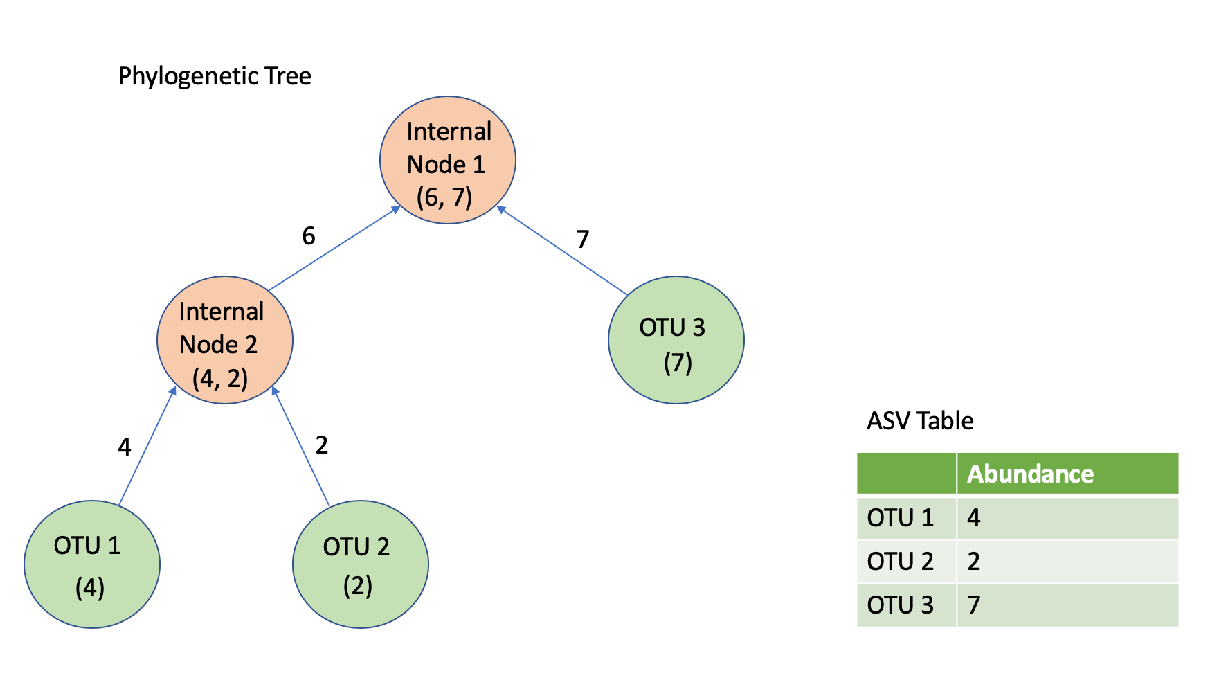
Figure 5.1: An example of bottom-up propagation of abundance counts

In addition to calculating counts going left and right at each internal node, code was also written in Python to determine the taxonomic rankings of each internal node, based upon the assigned taxonomies from the RDP for each ASV column in the sequence table. Figure 5.2 provides a smaller example of this propagation process.

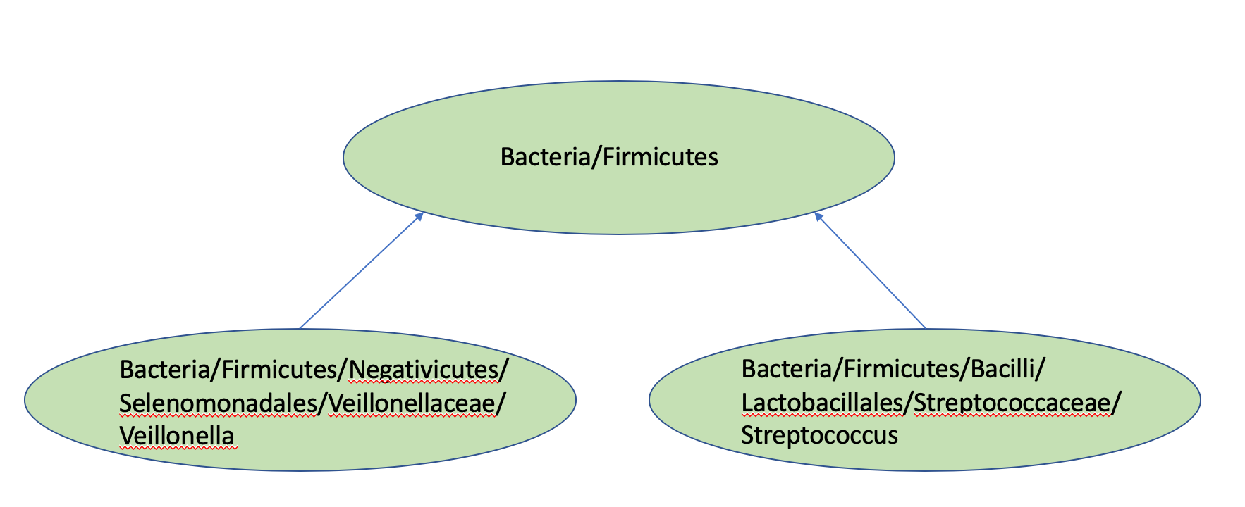
Figure 5.2: An example of bottom-up propagation of Taxonomies

With calculated counts and taxonomies for each of the internal nodes of our phylogenetic tree, we then fit a logit mixed-effect binomial model to each node, using the “glmer” function of the R “lme4” package (Bates, Machler, Bolker, & Walker, 2015). At each node, we had 370 observations after filtration for missing values. There were a total of 129 different patients in our dataset. We incorporated a random effect for patient ID, and a nested random effect within patient ID for sample date. We also included fixed effects for batch number, transplant age, gender, ethnicity, diagnosis, transplant type, graft source, vital status, care environment, presence of acute graft versus host disease, presence of chronic graft versus host disease, number of days post transplant that the ANC value is greater than 500, and “preOrPost,” telling us if the first sample was taken before or after the transplant date.

The general format of our mixed effects model is as follows:

\(logit(P_{i}(A)) = X_{i}\beta^{(A)} + \gamma_{i}^{(A)} + \epsilon_{it}^{(A)}\)

\(P_{i}(A)\) is the probability of picking the left child of node A for sample \(i\) at time \(t\).

\(\gamma_{i}^{(A)} = N(0, \sigma_{\gamma}^{2})\)

\(\epsilon_{i}^{(A)} = N(0, \sigma_{\epsilon}^{2})\)

\(for \ i = 1,...,370\)

In most cases, the regression model would fail to converge and provide meaningful results. However, there were twenty-two different internal nodes for which our model finished running and identified different variables to be significant.

Due to the fact that we had performed multiple tests, we applied a Bonferroni correction to our 22 nodes, requiring a p-value smaller than \(.05/22 = 2.27 * 10^{-3}.\) We settled on Bonferroni correction over other approaches to handling the multiple testing process due to how few of our nodes yielded successful regressions. With a success rate of just roughly 0.2%, Bonferroni correction helps us feel more certain that the variables we identify are indeed significant. In the future, we may choose to consider other forms of False Discovery Rate-controlling procedures, which would be less severe but still sufficiently accurate.

In addition to identifying several batch effects, we found significant variables for five of our nodes, with three significant variables found for the root node of our tree, and a single significant variable found for each of the other nodes. Figure 5.3 provides a table of the results of our phylogenetic tree decomposition, including the node number (higher numbers appear lower in the tree), the node taxonomy, the taxonomy of the children, the variable identified to be significant, estimates, and p-values.

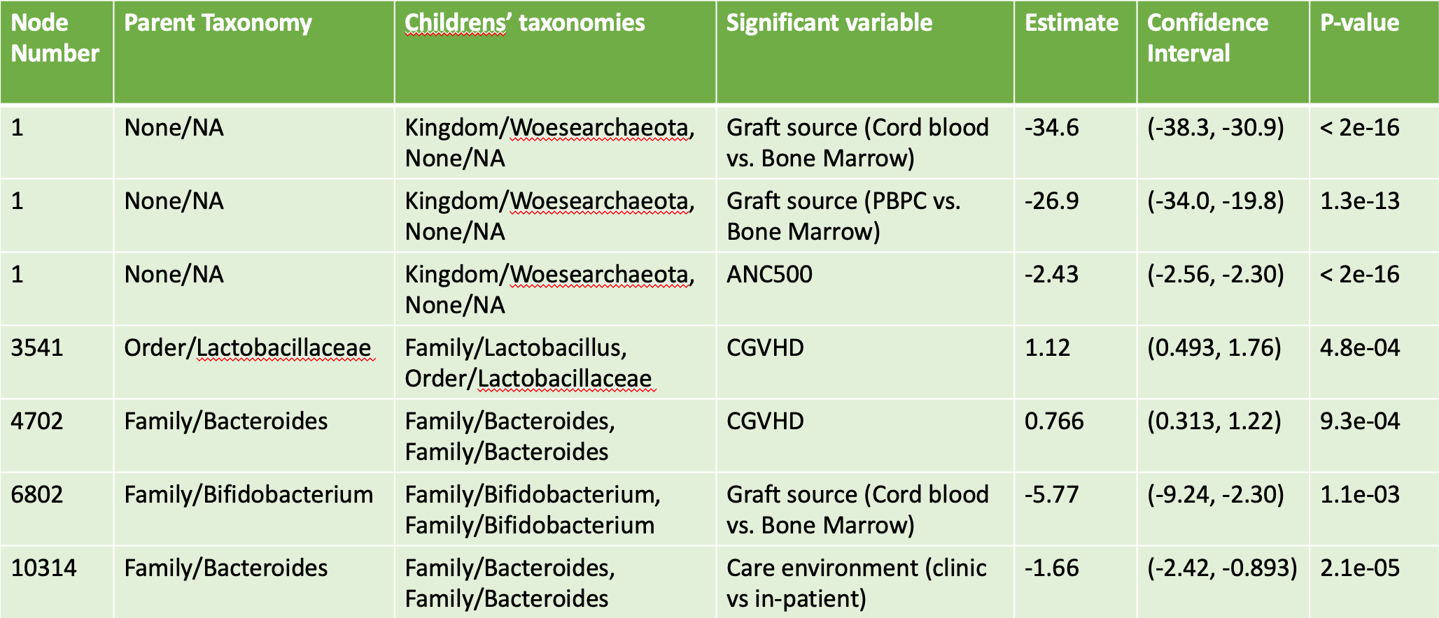
Figure 5.3: Significant Results from Phylogenetic Tree Decomposition after Bonferroni Correction

These results give us a bit of insight into the relationship between taxonomies and our covariates. For instance, interpreting the result for node 3541, we can say the following:

At this node, for a given stool sample and patient, and holding all else constant, having chronic graft versus host disease changes the odds for an ASV in the sample to belong in the more refined Lactobacillus Family compared to the more general Lactobacillaceae Order by a multiplicative factor of roughly 3.06 (confidence interval of [1.64, 5.81]).

Indeed, this output suggests a potential connection between CGVHD and microbiota in the lactobacillus family. We see that results for other nodes are a bit more difficult to interpret, because of the fact that parents and children have the same taxonomic classifications. Nevertheless, Phylogenetic Tree Decomposition offers a unique way to consider the effects of various covariates across different taxonomic levels. If we have varying taxonomies between the two children of a node, then being able to comprehend the odds of going left versus right given a certain value for a covariate will have greater meaning. If we were also able to perform analysis on full chains of internal nodes, then we could better identify the exact distributions of ASV counts across taxonomic groupings.