Chapter 1 Pre-processing of Microbiome Sequencing Data

Microbiome data can be procured from a multitude of sample types, including skin, the vagina, and the gut. Taken immediately from a sequencing experiment, microbiome data start off simply as a collection of FASTQ reads, each representing different bacterial sequences identified within the sample.

Filtration and clustering of these reads is required to produce a representation of microbiome data that can be effectively used for data analysis. The classic format of these processed data is known as the Operational Taxonomic Unit (OTU) table. These tables group DNA sequences into “molecular operational taxonomic units, clusters of sequencing reads that differ by less than a fixed dissimilarity threshold” (Callahan, McMurdie, Paul, & Holmes, 2017). Each row in the table represents a sample, each column represents a different OTU, and each value represents the abundance of the specific OTU within the sample. In the past couple of years, new methods have allowed researchers to work with amplicon sequence variants (ASVs) instead of OTUs. ASV groupings can be “resolved exactly, down to the level of single-nucleotide differences over the sequenced gene region,” allowing for improved resolution of processed data (Callahan et al., 2017). The DADA2 pipeline in R can be used to process microbiome sequence data and create an ASV table, yielding “more real variants and output[ting] fewer spurious sequences than other methods” (Callahan et al., 2016a).

As an exploration of the use of the DADA2 pipeline for the processing of microbiome sequencing data, we used the European Nucleotide Archive (Harrison et al., 2019) to download raw read data from Lozupone et al.’s 2013 study on gut-linked diseases prevalent in HIV (Lozupone et al., 2013). With these data, we applied Callahan et al.’s 2016 paper, “Bioconductor Workflow for Microbiome Analysis: from raw reads to community analyses,” to manipulate the Lozupone sequencing data. Using this pipeline, we visualized the fastq quality scores of our read files (Figure 1.1) to trim our input reads at ideal positions. We also filtered reads through the enforcement of a maximum threshold of two expected errors per read, as done in (Callahan et al., 2016a).

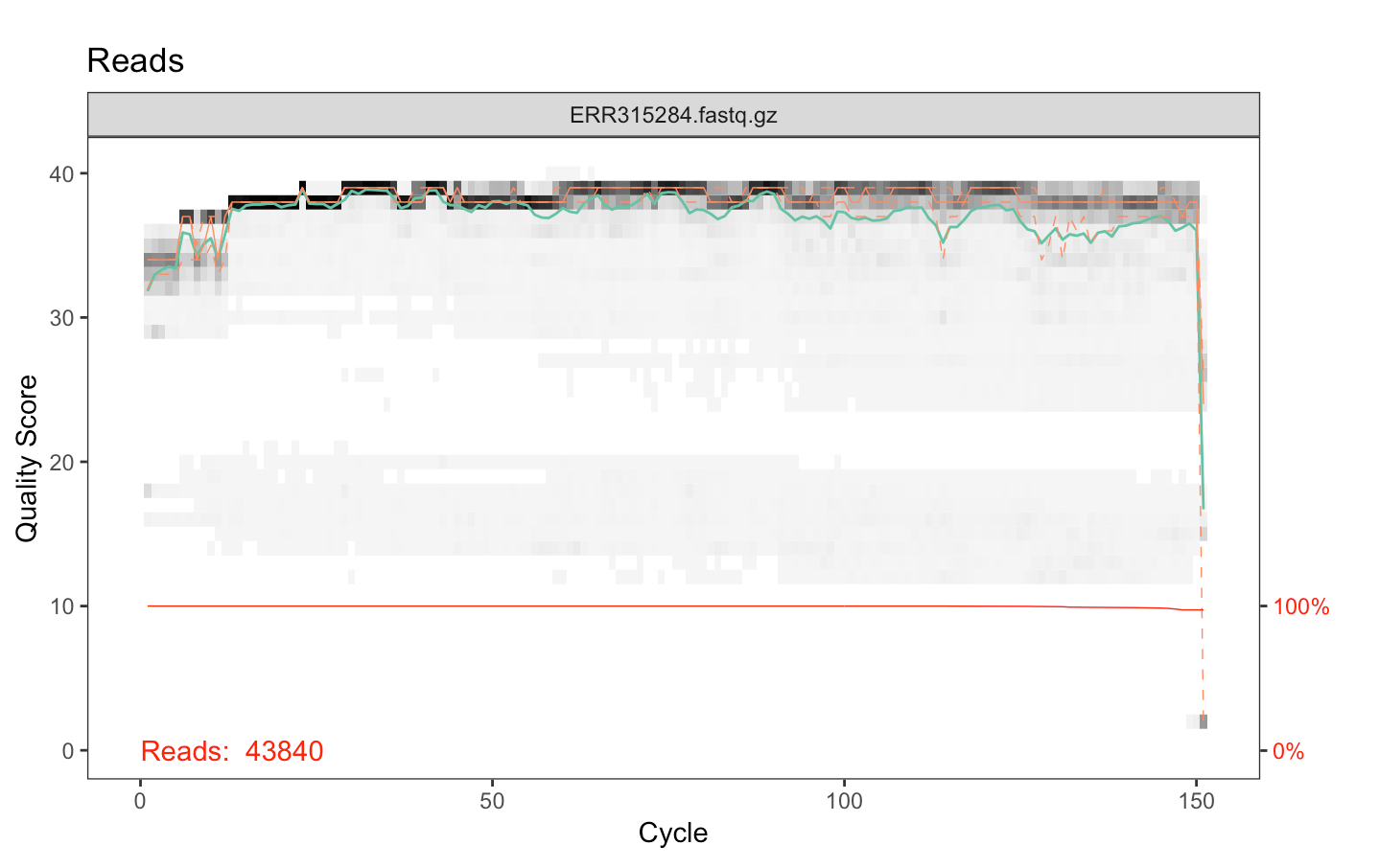
Figure 1.1: Fastq quality scores for a sample read file

Following the filtration of input reads, we used DADA2 to infer ASVs. Demultiplexed, dereplicated fastq files were selected for each sample. A sufficiently large subset of our data was taken, and then the DADA2 iterative sequence inference algorithm was run to estimate error rates and better resolve differences between sequences. We inspected the fit between observed error rates and fitted error rates to verify that our estimations were reasonable (Figure 1.2).

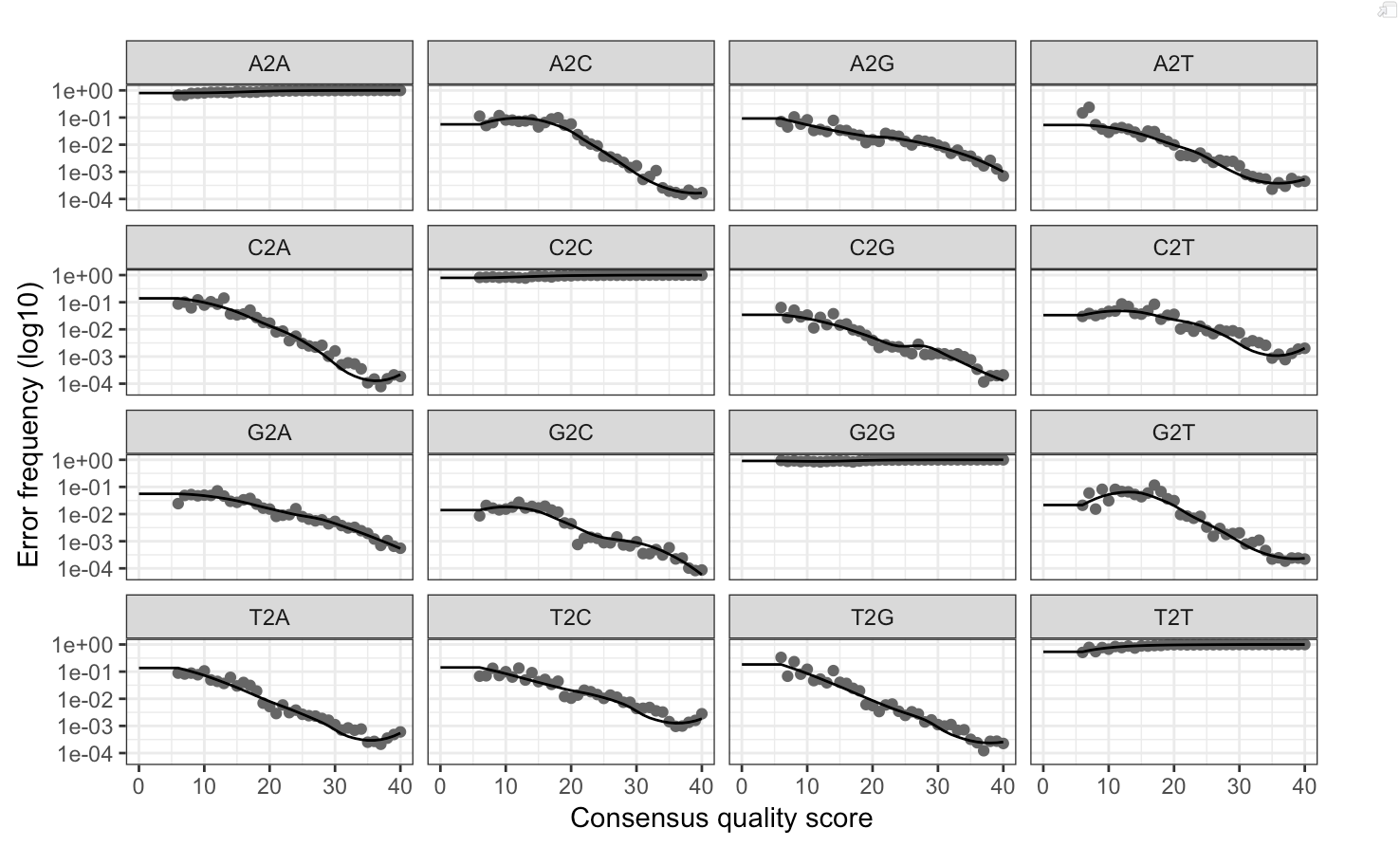
Figure 1.2: Comparison of observed and fitted error rates from the DADA2 iterative sequence inference algorithm

Using inference on pooled sequencing reads from all samples, DADA2 then removed nearly all substitution and insertion-deletion errors from our data. Finally, DADA2’s divisive partitioning algorithm was applied to create the distinct ASV clusters and generate a sequence table.

In a similar manner to how we were processing sequencing data for the Lozupone dataset, Alex Sibley, a bioinformatician working with the Sung lab in the Duke Cancer Institute, created an ASV table using the Memorial Sloan Kettering leukemia sequence reads. Given these data, we continued through the Callahan workflow to further filter and process our data.