Chapter 6 Pooled Analysis
We estimated the model coefficients of each completed dataset and conducted model diagnostic based on one completed dataset. We then combined model results of all datasets for inference.
6.1 Estimates of model coefficients
In a frequentist setting, estimates of model coefficients are computed through maximum likelihood estimation. In a Bayesian setting, estimates of model coefficients are computed through posterior distribution, which requires the specification of prior distributions.
Prior to seeing the data, we assumed that the intercept (\(\beta_{0}\)) have normal distribution with mean -3 and variance 2. The coefficients of the predictors (\(\beta = \beta_{1}, ..., \beta_{17}\)) have normal distribution with mean 0 and variance 5 - that \(\beta\) are as likely to be positive as they are to be negative but unlikely to be far away from zero. After observing the data, we modeled the likelihood of each observation as a binomial distribution \(p(y_{i}|x_{i},\beta_{0},\beta_{1},...,\beta_{17}) = Binomial(1, \pi_{i})\) for \(i = 1,...,n\); \(\pi_{i}\) is the probability of getting promoted, where \(\pi_{i} = logit^{-1}(\beta_{0} + \beta \cdot x_{i}) = \dfrac{exp(\beta_{0} + \beta \cdot x_{i})}{1 +exp(\beta_{0} + \beta \cdot x_{i}) }\). The posterior distribution is proportional to the product of the priors and the likelihood distribution. To sum up, the posterior distribution is derived as below.
Prior Distribution \[ \begin{aligned} f(\beta_{0}) &= N(-3,2)\\ f(\beta_{k}) &= N(0,5), k = 1,...,17 \\ \end{aligned} \]
Likelihood \[ \begin{aligned} p(Y|x^{cmp},\beta_{0},\beta) & = \prod_{i=1}^{n} p(y_{i}|x_{i},\beta_{0},\beta) \\ & = \prod_{i=1}^{n} [logit^{-1}(\beta_{0} + \beta \cdot x_{i})]^{y_{i}}[1 - logit^{-1}(\beta_{0} + \beta \cdot x_{i})]^{(1-y_{i})}\\ \end{aligned} \]
Posterior Distribution \[ \begin{aligned} f(\beta_{0},\beta|X,Y) & = f(\beta_{0}){\prod_{k=1}^{17} f(\beta_k)} f(Y|x^{cmp},\beta_{0},\beta) \\ & \propto f(\beta_{0}) {\prod_{k=1}^{17} f(\beta_k)} [\prod_{i=1}^{n} logit^{-1}(\beta_{0} + \beta x_{i})]^{y_{i}}[\prod_{i=1}^{n}(1- logit^{-1}(\beta_{0} + \beta x_{i}))]^{(1- y_{i})} \end{aligned} \]
Model Diagnostic
Logistic regression does not require the assumptions of constant variance and normality of residuals. To check if the predictors of fitted logistic regression model are well specified, we applied binned residuals technique. The procedures to produce binned residuals include: first, we computed raw residuals of the fitted model and ordered observations by values of predicted probabilities; second, for continuous predictor, we formed \(\sqrt{27346} \approx 165\) equally sized, ordered bins using the ordered data and computed average residual of each bin. Next, we plotted average residual versus average predicted probability of each bin to check if there are any specific patterns that might cause problems; third, for categorical predictor, we computed average residual of each level.
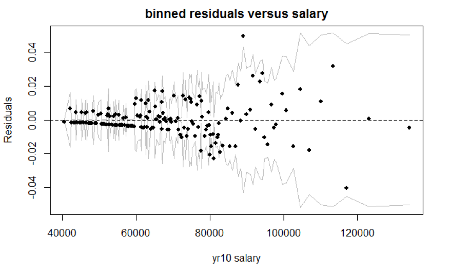
Figure 6.1: Residuals Binned Plot
We created the binned residuals plot (Figure 6.1) based on one imputed dataset’s model (Frequentist model) results. The average residuals are close to 0 for salary less than $82,425, but tend to fluctuate for salary greater than $82,425. That data with higher salary values are more sparse leads to the fluctuation. For categorical variable, the number of level is limited and majority of the time the prediction would yield 0 (not promoted), and thus, the average residuals for each bin are small. In general, we did not observe extreme residuals, but we should be wary of data with higher salary values.
| M | F |
|---|---|
| \(-1.473e^{-10}\) | \(-1.916e^{-10}\) |
| P | A | O |
|---|---|---|
| \(-8.481e^{-11}\) | \(-2.158e^{-10}\) | \(-2.186e^{-10}\) |
| B | A | C | D | E |
|---|---|---|---|---|
| \(1.847e^{-10}\) | \(-2.093e^{-10}\) | \(-1.351e^{-10}\) | \(-3.733e^{-11}\) | \(-2.573e^{-11}\) |
| White | Non-white |
|---|---|
| \(1.570e^{-10}\) | \(-1.869e^{-10}\) |
| Switch | No-switch |
|---|---|
| \(-1.549e^{-10}\) | \(-1.658e^{-10}\) |
| Supervisor | Non-supervisor |
|---|---|
| \(-2.010e^{-10}\) | \(-1.588e^{-10}\) |
| Grade0 | Grade1 | Grade2 |
|---|---|---|
| \(-2.464e^{-10}\) | \(-5.606e^{-12}\) | \(-5.440e^{-12}\) |
| Change2 | Change1 | Change3 |
|---|---|---|
| \(-1.888e^{-10}\) | \(-1.184e^{-10}\) | \(-1.351e^{-10}\) |
6.2 Pooled results
We combined poole results for both Frequentist model and Bayesian model. For Frequentist model, we obtained the pooled results through (1) averaging out the estimated regression coefficients of each completed dataset (2) accounting for both within and across datasets variances. For Bayesian model, we obtained the pooled results through summarizing the mixture draws from posterior distribution.
6.2.1 Frequentist model
For each completed dataset \(j\) (\(j = 1,...,12\)) and each regression coefficient \(\beta_{ij}\) (\(i = 0,...,17\)), let \(q_{ij}\) be the estimator of \(\beta_{ij}\) from \(j_{th}\) dataset, and let \(u_{ij}\) be the estimator of the variance of \(\beta_{ij}\) from \(j_{th}\) dataset. First, we computed the average of each dataset’s estimated slope to obtain the estimate of the model coefficient \(\overline{q_{i}}\). Second, we computed the average of each dataset’s estimated slope variance to obtain the within-dataset variance \(\overline{u_{i}}\). Thid, we computed the variance of the slopes across 12 datasets to obtain the across-datasets variance \(b_{i}\).
\[ \begin{aligned} & \overline{q_{i}} = \sum_{j=1}^{12}q_{ij}/12 \\ & \overline{u_{i}} = \sum_{j=1}^{12}u_{ij}/12 \\ & b_{i} = \sum_{j=1}^{12}(q_{ij} -\overline{q_{i}})/(12-1) \\ \end{aligned} \]
With average estimated regression coefficient (\(\overline{q_{i}}\)), within-dataset variance (\(\overline{u_{i}}\)), and across-datasets variance (\(b_{i}\)), the point estimate of \(\beta_{i}\) is \(\overline{q_{i}}\), and its variance is \(T_{i} = (1+1/12)b_{i}+\overline{u_{i}}\). An approximate 95% confidence interval is \(\overline{q_{i}} \pm 1.96\sqrt{T_{i}}\). The table below shows the pooled estimated slope, standard error, and 95% confidence interval of each regression coefficient.
| Coefficient | Estimate | Std. Error | 95% CI. |
|---|---|---|---|
| Intercept (\(\beta_{0}\)) | -6.018 | 0.697 | [-6.871, -5.164] |
| Female (\(\beta_{1}\)) | -0.035 | 0.012 | [-0.0815, 0.011] |
| OccA (\(\beta_{2}\)) | 0.744 | 0.015 | [0.709, 0.779] |
| OccO (\(\beta_{3}\)) | 1.005 | 0.299 | [0.845, 1.170] |
| EducA (\(\beta_{4}\)) | -0.712 | 0.036 | [-0.748, -0.675] |
| EducC (\(\beta_{5}\)) | 0.128 | 0.016 | [0.094, 0.161] |
| EducD (\(\beta_{6}\)) | 0.195 | 0.033 | [0.139, 0.252] |
| EducE (\(\beta_{7}\)) | -0.047 | 0.045 | [-0.129, 0.036] |
| Non-white (\(\beta_{8}\)) | -0.112 | 0.017 | [-0.151, -0.074] |
| No-switch (\(\beta_{9}\)) | -0.039 | 0.031 | [-0.057, -0.020] |
| Non-Supervisor (\(\beta_{10}\)) | -0.949 | 0.013 | [-1.008, -0.890] |
| Grade0 (\(\beta_{11}\)) | -0.450 | 0.066 | [-0.657, -0.244] |
| Grade2 (\(\beta_{12}\)) | 1.389 | 0.049 | [1.213,1.565] |
| ScaledSalary (\(\beta_{13}\)) | 1.939 | 0.618 | [1.157, 2.721] |
| (ScaledSalary + 1.0751) (\(\beta_{14}\)) | 2.919 | 0.642 | [2.077, 3.761] |
| (ScaledSalary - 0.2272) (\(\beta_{15}\)) | 3.328 | 0.902 | [2.362, 4.294] |
| Change1 (\(\beta_{16}\)) | -0.266 | 0.027 | [-0.457, -0.074] |
| Change3 (\(\beta_{17}\)) | 0.233 | 0.025 | [0.065, 0.401] |
6.2.2 Bayesian Model
For Bayesian model, instead of averaging out the estimated regression coefficients, we obtained the pooled results through applying the approach proposed by Zhou and Reiter (2010). For each completed dataset \(l = 1,...,m\) and parameter of interest \(Q\), denote \(Q^{(l)}\) as the MCMC draws from posterior distribution. First, simulate \(J\) values of posterior draws (where \(J\) is large) from each \(Q^{(l)}\), with its distribution denoted as \(\hat{f}(Q^{(l)})\). Second, mix all \(\hat{f}(Q^{(l)})\) to form \(\hat{f}(Q^{(all)})\). Third, sort total number of \(m*J\) draws from \(\hat{f}(Q^{(all)})\), where the estimates of 95% posterior interval, posterior median, and other statistics can be obtained from the mixed posterior draws (Zhou & Reiter, 2010).
The pooled estimated slope, standard error, and 95% credible interval are generated through specifying \(J = 4000\) to create a total number of \(12*4000 = 48000\) draws. The table below shows the pooled estimated slope, standard error, and 95% credible interval of each regression coefficient.
| Coefficient | Estimate | Std. Error | 95% CI. |
|---|---|---|---|
| Intercept (\(\beta_{0}\)) | -6.033 | 0.816 | [-7.732, -4.529] |
| Female (\(\beta_{1}\)) | -0.036 | 0.110 | [-0.254, 0.176] |
| OccA (\(\beta_{2}\)) | 0.745 | 0.124 | [0.502, 0.988] |
| OccO (\(\beta_{3}\)) | 0.877 | 0.571 | [-0.359, 1.887] |
| EducA (\(\beta_{4}\)) | -0.719 | 0.191 | [-1.103, -0.354] |
| EducC (\(\beta_{5}\)) | 0.127 | 0.127 | [-0.123, 0.375] |
| EducD (\(\beta_{6}\)) | 0.190 | 0.183 | [-0.174, 0.542] |
| EducE (\(\beta_{7}\)) | -0.056 | 0.212 | [-0.479, 0.355] |
| Non-white (\(\beta_{8}\)) | -0.116 | 0.132 | [-0.383, 0.140] |
| No-switch (\(\beta_{9}\)) | -0.029 | 0.178 | [-0.365, 0.326] |
| Non-Supervisor (\(\beta_{10}\)) | -0.950 | 0.112 | [-1.167, -0.729] |
| Grade0 (\(\beta_{11}\)) | -0.458 | 0.253 | [-0.966, 0.025] |
| Grade2 (\(\beta_{12}\)) | 1.395 | 0.218 | [0.969, 1.823] |
| ScaledSalary (\(\beta_{13}\)) | 1.933 | 0.770 | [0.530, 3.559] |
| (ScaledSalary + 1.0751) (\(\beta_{14}\)) | 2.915 | 0.781 | [1.476, 4.538] |
| (ScaledSalary - 0.2272) (\(\beta_{15}\)) | 3.316 | 0.927 | [1.573, 5.205] |
| Change1 (\(\beta_{16}\)) | -0.268 | 0.159 | [-0.586, 0.032] |
| Change3 (\(\beta_{17}\)) | 0.231 | 0.154 | [-0.078, 0.521] |
6.2.3 Comparison between Frequentist and Bayesian Model
We compared the pooled results for both Frequentist model (Figure 6.2) and Bayesian model (Figure 6.3). The pooled coefficient means of both models are close to each other, but Bayesian model has higher pooled standard errors. There are certain requirements for Bayesian inference after multiple imputation. Our inherent constraints - prior parameter choices and number of available imputed datasets therefore lead to greater uncertainty. First, the posterior distribution depends on the choice of prior parameter, which usually requires knowledge from experts. Our choice of non-informative prior might not be the most ideal prior. Second, Zhou and Reiter (Zhou & Reiter, 2010) suggested that the number of imputed datasets should be large (at least 100 imputed datasets) in order for Bayesian inference to work well. Since there are only 12 available imputed datasets, Bayesian inference might not be valid. Thus, we conducted inference based on the Frequentist model.
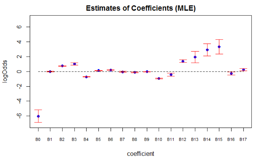
Figure 6.2: Frequentist Model
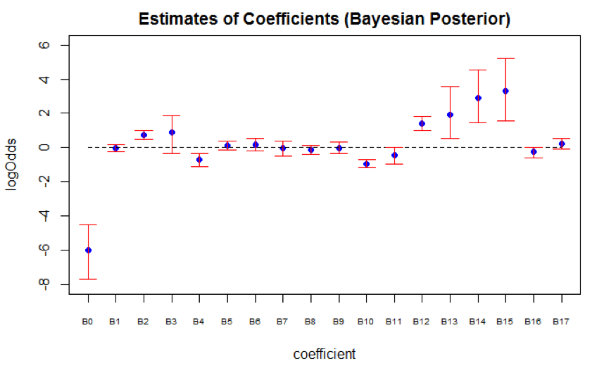
Figure 6.3: Bayesian Model
6.3 Inference based on Frequentist model
In general, the selection of the SES positions is highly dependent on (1) personal skills (indicated by variable Occupational Category and Supervisory Status) (2) education level (indicated by variable Education Group) and (3) performance at work (indicated by variable Salary, Grade, and Change in Pay Rate)
First, for employees whose occupational category are Administrative, the odds of getting promoted are multiplied by a factor of 2.104 (95% CI: 2.031 to 2.180) compared to employees whose occupational category are Professional, holding all else constant. This implies that analytical ability, judgment, discretion, and personal responsibility (characteristics of occupational category Administrative) might be more important than having knowledge in a specific field of science (characteristics of occupational category Professional). Furthermore, for employees who do not serve in supervisory positions, the odds of getting promoted are multiplied by a factor of 0.387 (95% CI: 0.365 to 0.411) than employees who serve in supervisory positions, holding all else constant. Since leadership is one of the key competencies for the SES positions, employees without leadership experiences might be put into disadvantages.
Second, education level also plays an important role when it comes to predicting promotion outcome. For employees with degrees below Bachelor’s, the odds of getting promoted is multiplied by 0.491 (95% CI: 0.473 to 0.509) compared to employees with Bachelor’s degree, holding all else constant. Furthermore, though it is expected that the odds of getting promoted would increase with higher education level, there is certain limit. Specifically, compared to employees with only Bachelor’s degrees, the odds of getting promoted increases if employees acquired Master’s and Advanced degrees. However, the effect of PhD degrees on predicting promotion is not significant because its 95% confidence interval contains 0. Because PhD degrees focus on particular fields of studies, this result further confirms that having specific knowledge in a field of science might not be one of the important promotion criteria.
Third, compared to employees with grade 13 and 14 at working year 10, the odds of getting promoted are multiplied by a factor of 0.637 (95% CI: 0.519 to 0.784) for employees with grade below 13, but multiplied by a factor of 4.010 (95% CI: 3.364 to 4.781) for employees with grade 15. The visualization graphs further show the relationship between salary at given grade and % change in salary (Grade 15 for Figure 6.4, Grade 14 for Figure 6.5, Grade 13 for Figure 6.6, Grade < 13 for Figure 6.7). Regardless of Grade, the predicted probability of getting promoted increases as salary increases, and employees with bigger percentage change in salary also have higher odds of getting promoted. Note that the model yields predicted probability up to 0.25 at Grade 15. Given the small proportion of ones, we believe that the predicted probability at grade 15 is potentially overestimated due to sparsity of the data at higher salary values.
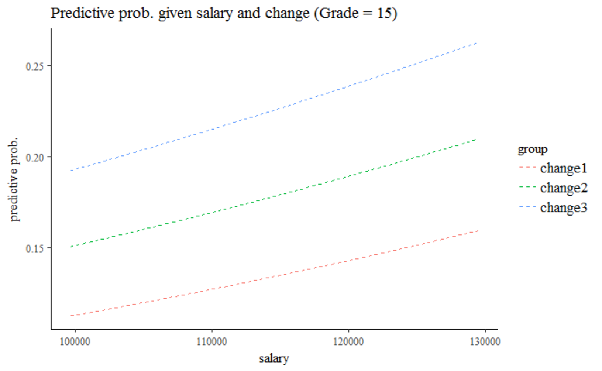
Figure 6.4: Grade 15
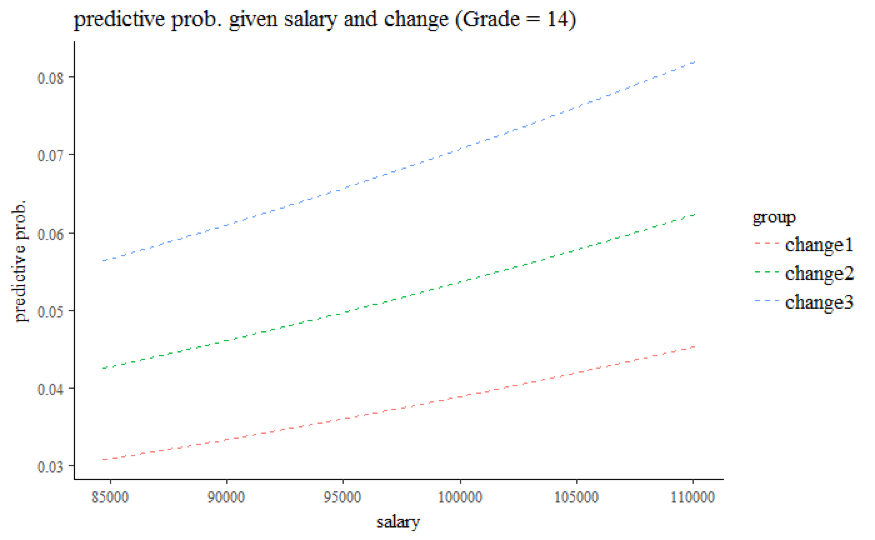
Figure 6.5: Grade 14
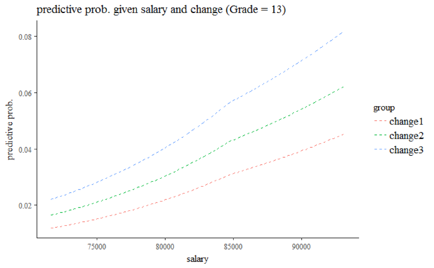
Figure 6.6: Grade 13
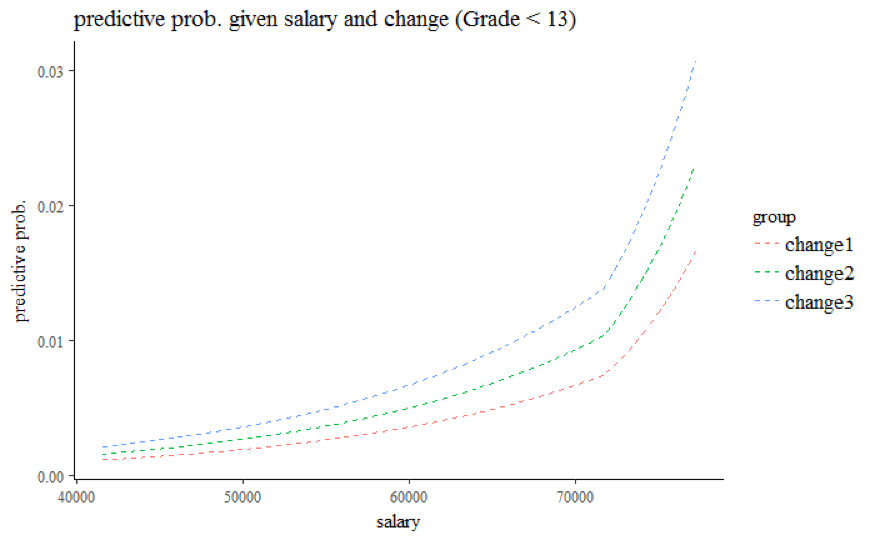
Figure 6.7: Grade < 13
Lastly, the 95% confidence interval of variable Gender contains value 0, suggesting that the effect of Gender is not significant in predicting promotion outcome. For employees whose race are Non-white, the odds of getting promoted are multiplied by a factor of 0.894 (95% CI: 0.868 to 0.929) compared to employees whose race are White, holding all else constant.
6.4 Conclusion and future improvement
In conclusion, the model suggests an employee’s personal skills and performance at work are significant in predicting promotion outcomes, but certain limitations exist for the model. First, the analysis is based on 10% samples of the OPM data, and we would like to apply the current model to the full samples. Second, the predictive probability of employees with very high salary values is potentially overestimated because the piecewise linear model is not granular enough to account for small proportion of ones in outcome variables. In the future, we would like to experiment on various models to improve the predictive accuracy. Third, we did not have enough imputed datasets to account for random noises produced by the imputation models. This also affected the validity of the Bayesian inference after multiple imputation. In the future, we would like to impute more completed datasets through expanding computational capacity.