Chapter 4 Exploratory Data Analysis (EDA)
After checking the robustness of the imputation model, we conducted exploratory data analysis and model fitting based on one imputed dataset.
4.1 Outcome variable and covariates selection
Outcome Variable
Variable Promoted is the outcome variable, indicating whether an employee was promoted into the SES position after working year 10 (1 = promoted, 0 = not promoted). In order for the analysis to be consistent, we only included employees with GS or GM pay plan. 482 out of 27,932 employees were promoted.
Covariates
The OPM data contain detailed information about the federal employees, but some variables are unrelated to the goal of the study. Based on past social science research on the selection of high-level executives within both private and public sectors, we logically chose variables relevant to our questions of interests as covariates.
First, Gender could be a predictor as past studies have shown that gender plays an important role in the promotion of high-level executives. For example, the glass ceiling phenomenon, the phenomenon that keeps women from reaching the top level of organizations, exists in both public and private sectors (Powell & Butterfield, 1994). Second, Race and Education Level are important predictors for federal employees’ salary information (Barrientos et al., 2017), and could potentially impact the promotion process. Both variables should be included as covariates.
Third, employees with the SES position are required to build coalitions both within and outside the organizations. We extrapolated that employees who had experiences working in various government agencies might possess this competency. Department Switch, a variable indicating whether an employee switched department between working year 1 and working year 10, could be a critical predictor. Fourth, senior executives are often tasked to lead people and make strategic changes, and variables such as Occupational Category and Supervisory Status might provide pertinent information.
Lastly, the promotion criteria depend on an employee’s performance at work. There is a formal appraisal system in the OPM, but such system was not established until 1996. Given the timeframe of the studies (employees starting between 1978 and 1997), it is not appropriate to include this variable. To address this problem, we decide to include Salary and Grade at working year 10 because these variables could potentially indicate an employee’s mid-career performance. Furthermore, we create an additional covariate Change in Pay Rate, which specifies an employee’s rate of change in salary between working year 1 and working year 10. Particularly, we posited that higher rate of change in salary would indicate better work performance.
Assumptions
The number of the SES position is limited in each agency and potential candidates tend to get promoted at different year. Though the promotion criteria might vary among years, we had to make one key assumption given the rarity of the total number of positions. That is, the covariates selected are general enough to capture the promotion criteria despite time differences. Furthermore, we adjusted salary information in terms of 2011 inflation rate to ensure we could compare variables dependent on time on the same basis.
4.2 Inspection of each covariate
We examined the relationship between outcome variable and predictors with two strategies. First, for categorical predictors, we looked at the percentages of ones in outcome variable for each level. If a categorical predictor has many levels but the percentages of ones in outcome variable for certain levels is limited, we considered regrouping to reduce levels. Second, for continuous predictor, we broke predictor into \(n\) equally sized, ordered groups, and computed the percentage of ones in outcome variable for each group. We then visualized the patterns between groups and explored the needs for transformation.
Gender (Categorical)
Variable Gender has 2 levels - Male and Female (M,F). There are more females than males, but each gender has similar proportion of ones.
| Gender | population (%) | promoted (%) |
|---|---|---|
| Male (M) | 39.62 | 1.39 |
| Female (F) | 60.38 | 1.76 |
Race (Categorical)
Variable Race has 6 levels - Hispanic or Latino (1), American Indian or Alaska Native (2), Asian (3), Black or African American (4), Native Hawaiian or Other Pacific Islander (5), and White (6). Because there are significantly less people with race level (1) to (5) than people with race level (6), it is regrouped into two levels - Non-white (0), and White (1).
| Race | population (%) | promoted (%) |
|---|---|---|
| Hispanic/Latino (1) | 7.65 | 0.91 |
| American Indian/Alaska Native (2) | 1.70 | 1.07 |
| Asian (3) | 4.46 | 0.82 |
| Black/African American (4) | 12.43 | 1.38 |
| Native Hawaiian/Other Pacific Islander (5) | 0.05 | 0 |
| White (6) | 73.69 | 1.79 |
| Race | population (%) | promoted (%) |
|---|---|---|
| Non-white (0) | 26.30 | 1.13 |
| White (1) | 73.69 | 1.79 |
Education Level (Categorical)
Variable Education Level has 7 levels - High School Degree or less (0), More than High School, No Bachelor’s (1), Bachelor’s (2), Master’s (3), Professional Degree (4), Advanced Certification (5), and PhD (6). Because certain education levels have relatively small population size, it is regrouped from 7 to 5 levels based on each level’s characteristics: employees without Bachelor’s degree (level (0) and level (1)) are combined into one group, and employees with Professional Degree and Advanced Certification (Level (4) and (5)) are combined into another group.
| Education Level | population (%) | promoted (%) |
|---|---|---|
| High School Degree or less (0) | 8.56 | 0.38 |
| More than High School, No Bachelor’s (1) | 18.57 | 0.59 |
| Bachelor’s (2) | 40.44 | 1.39 |
| Master’s (3) | 22.33 | 2.31 |
| Professional Degree (4) | 5.05 | 4.78 |
| Advanced Certification (5) | 0.25 | 1.45 |
| PhD (6) | 4.79 | 3.05 |
| Education Level | population (%) | promoted (%) |
|---|---|---|
| Less than Bachelor’s (A) | 27.14 | 0.53 |
| Bachelor’s (B) | 40.44 | 1.39 |
| Master’s (C) | 22.33 | 2.31 |
| Professional Degree & Advanced Certification (D) | 5.30 | 4.62 |
| PhD (E) | 4.79 | 3.05 |
Department Switch (Categorical)
Variable Department Switch indicates whether employees switch department between working year 1 and working year 10. The majority did not switch department. Regardless of department switch, each group has similar proportion of people promoted into the SES position.
| Department Switch | population (%) | promoted (%) |
|---|---|---|
| No Switch | 91.17 | 1.6 |
| Switch | 8.83 | 1.7 |
Occupational Category (Categorical)
Variable Occupational Category has 3 levels - Administrative (A), Professional (P), and Other White Collar (O).
| Occupational Category | population (%) | promoted (%) |
|---|---|---|
| Administrative (A) | 58.06 | 1.71 |
| Professional (P) | 38.97 | 1.56 |
| Other (O) | 2.97 | 0.49 |
Supervisory Status (Categorical)
Variable Supervisory Status indicates whether employees hold supervisory position at working year 10. Employees with supervisory positions have higher proportion of ones than people without supervisory positions.
| Supervisory Status | population (%) | promoted (%) |
|---|---|---|
| Supervisor | 14.34 | 5.69 |
| Non-supervisor | 85.66 | 0.93 |
Year 10 Grade (Categorical)
Variable Year 10 Grade consists of 7 levels - grade 9 - 15. The proportion of ones for grade 9 to 12 is small, but increases significantly for grade 13 to 15. It is regrouped into three levels - 0 (Grade 9 - 12), 1 (Grade 13 & 14), and 2 (Grade 15).
| Year 10 Grade | population (%) | promoted (%) |
|---|---|---|
| 9 | 16.46 | 0.11 |
| 10 | 2.44 | 0.30 |
| 11 | 22.88 | 0.26 |
| 12 | 24.35 | 0.75 |
| 13 | 20.81 | 1.69 |
| 14 | 9.66 | 4.77 |
| 15 | 3.39 | 15.73 |
| Year 10 Grade | population (%) | promoted (%) |
|---|---|---|
| 0 | 66.13 | 0.4 |
| 1 | 30.48 | 2.66 |
| 2 | 3.39 | 15.73 |
Year 10 Salary (Continuous)
Variable Year 10 Salary specifies employees’ salary at working year 10. Based on OPM’s 2011 General Schedule pay table, employees with grade 9 has minimum salary of $41,563, and employees with grade 15 has maximum salary of $129,517. Due to random noises produced by the imputation model, the imputed datasets consist of grade 9 employees with salary less than 41,563, and grade 15 employees with salary greater than 129,517. Since these outliers account for less than 0.1% of the total observations for each imputed dataset, no concerns on the robustness of the analysis are raised. In addition, combining multiple imputed datasets to form final analysis could help averaging out the random noises.
The visualization graph (Figure 4.1) is produced based on the strategy mentioned before. The x-axis denotes 10 equally sized group, with each group representing certain salary ranges. (Year 10 Salary Table). The y-axis denotes the percentage of ones in each group. In general, employees with higher salary have higher percentage of ones. Group 1 to 8 have percentage of ones less than 2 %, whereas group 9 and 10 have percentage of ones larger than 2 %. The flat curve between group 1 and group 8 and the spike in group 9 and 10 indicate that the relationship between outcome variable and year 10 salary predictor is non-linear. To capture the non-linear relationship, we considered various transformation such as quadratic polynomial transformation, and semi-parametric piecewise spline function is the most effective in modeling this continuous predictor. The detailed descriptions of spline modeling will be mentioned in the next section.
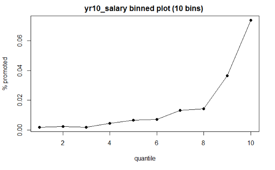
Figure 4.1: Year 10 Salary Binned Plot
| Group | Salary Range | % promoted |
|---|---|---|
| 1 | [25740,47744) | 0.18 |
| 2 | [47744,52653) | 0.22 |
| 3 | [52653,56801) | 0.18 |
| 4 | [56801,61726) | 0.44 |
| 5 | [61726,66339) | 0.66 |
| 6 | [66339,71136) | 0.69 |
| 7 | [71136,77180) | 1.3 |
| 8 | [77180,82160) | 1.43 |
| 9 | [82160,93591) | 3.65 |
| 10 | [93591,149505) | 7.39 |
Note that we recentered and rescaled the year 10 salary for interpretation purpose. First, year 10 salary is centered on the mean salary at grade 13 from OPM’s 2011 pay table (the mean is around $82,425). Second, it is also scaled by $10,000. Denote \(x_{i}\) as employee \(i\)’s year 10 salary, \(scale(x_{i}) = \dfrac{x_{i} - 82,425}{10,000}\).
Change in Pay Rate (Categorical)
Variable Change in Pay Rate specifies the change in pay rate between working year 1 and working year 10. The construction of the visualization graph for change in pay rate (Figure 4.2) is similar to that for year 10 salary. The x-axis denotes 10 equally sized group, with each group representing certain change in pay rate (Change in Pay Rate Table). The y-axis denotes the percentage of ones in each group. Though we believe that higher percentage of change in salary might indicate better performance at work, it is not reflected in the promotion of the SES position. Regardless of change rate, the graph does not indicate particular trend as the proportion of ones fluctuates among groups. This means that Change in Pay Rate probably does not provide predictive power if treated as continuous variable.
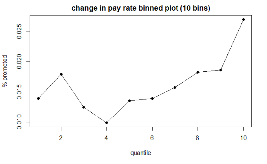
Figure 4.2: Change in Pay Rate Binned Plot
| Group | % Change Range | % promoted |
|---|---|---|
| 1 | [-10.3,40.4) | 1.39 |
| 2 | [40.4,57.2) | 1.79 |
| 3 | [57.2,69.8) | 1.24 |
| 4 | [69.8,81.1) | 0.10 |
| 5 | [81.1,92.5) | 1.35 |
| 6 | [92.5,105.5) | 1.39 |
| 7 | [105.5,120.5) | 1.57 |
| 8 | [120.5,140.7) | 1.83 |
| 9 | [140.7,174.8) | 1.87 |
| 10 | 174.8+ | 2.71 |
| Group | % Change Range | promoted (%) |
|---|---|---|
| Change1 | [-10.34,62) | 1.51 |
| Change2 | [62,160) | 1.42 |
| Change3 | 160+ | 2.66 |
To address the problem, we decide to model pay rate as a categorical variable with 3 levels. The first level consists of employees with rate changes below 62% (equals to around 5% change per year). This pay rate change range falls within the regular rate change of the federal government. The second level consists of employees with rate change between 62% and 160% (equals to around 5 - 10% change per year). This rate change range is higher than the regular rate change, indicating that employees with this rate change level might perform better than employees with regular rate change. The third level consists of employees with rate changes above 160%. This rate change is significantly higher than the regular change rate. Note that some of the very high rate change values are sensitive to the imputation models since more than 80% of the rate change data is missing.