Chapter 5 Model Fitting

5.1 Logistic regression with piecewise linear spline application

In Generalized Linear Models (GLMs), the relationship between coefficients of predictors and univariate outcome variable is usually linear. The binnedplot of variable Year 10 Salary in the previous chapter, however, indicates that the relationship between outcome variable and the predictor is non-linear. Incorporating smoothing techniques such as the application of spline function is a common strategy to model data with non-linear relationship (Walther, 2017). Specifically, we applied piecewise linear spline function to model the data.

To recap the relationship between predictor Year 10 Salary and outcome variable, the proportion of ones below certain salary level is relatively flat, whereas the proportion of ones above certain salary level increases significantly (Figure 5.1). This indicates that the coefficient slopes above and below certain salary level are different.

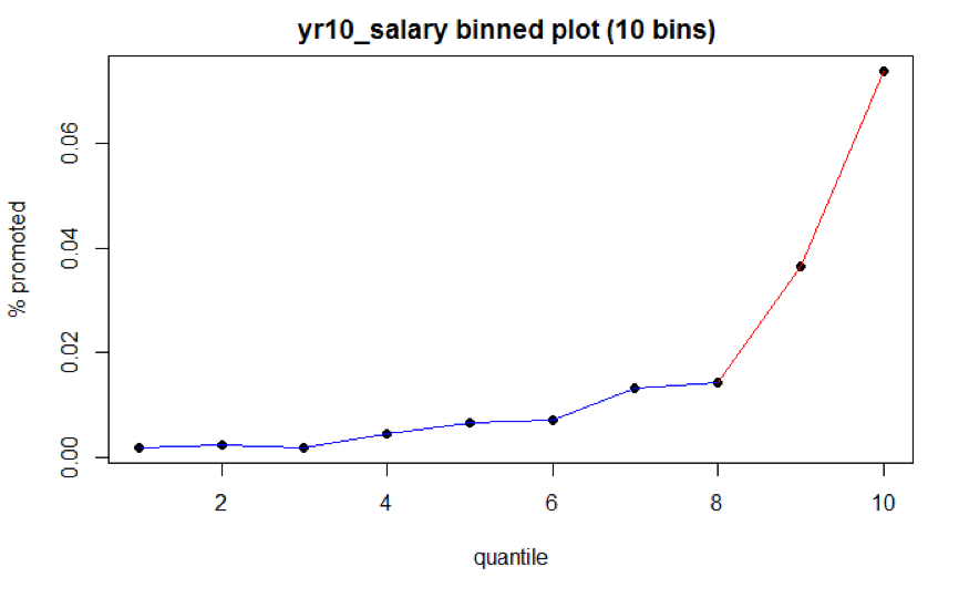
Figure 5.1: Year 10 Salary Binned Plot

A spline of degree \(D\) is a continuous function formed by connecting polynomial segments. The points where the segments connect are called the knots of the spline. In general, a spline of degree D associated with a knot \(\xi_{k}\) takes the form: \[ (x-\xi_{k})_{+}^{D}= \begin{cases} 0, & x < \xi_{k}\\ (x-\xi_{k})^{D}, & x \geq \xi_{k} \end{cases} \]

We created another binned plot with 25 bins (Fig 5.2) in order to select knots (\(\xi_{k}\)) granularly. The first knot is chosen as the cut point between black and blue segments, which takes the value of $71,674. Since year 10 salary is centered and scaled, this cut point should be \(\dfrac{71,674 - 82,425}{10,000} = -1.0751\). The second knot is chosen as the cut point between blue and red segments, which takes the value of $84,697 (\(\dfrac{84,697 - 82,425}{10,000} = 0.2272\)).

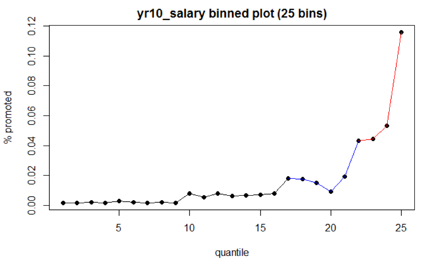
Figure 5.2: Year 10 Salary Binned Plot

Spline function with higher degree \(D\) can better capture the non-linear relationship. However, we found it inappropriate to model the OPM data with higher degree \(D\) due to the small proportion of ones in outcome variable. To avoid overfitting, we chose a degree \(D\) of 1 for the spline function.

To sum up, denote \(x\) as the year 10 salary after transformation. The prediction function for the piecewise linear spline is \[ \begin{aligned} & \beta_{0} + \beta_{1}x + \beta_{2}(x - (-1.0751))_{+} + \beta_{3}(x - 0.2272)_{+} \\ = & \beta_{0} + \beta_{1}x + \beta_{2}(x + 1.0751)(I[x \geq -1.0751]) + \beta_{3}(x - 0.2272)(I[x \geq 0.2272]) \end{aligned} \]

Specifically, if year 10 salary is below the first cut point, then coefficient \(\beta_{2}\) and \(\beta_{3}\) equals to 0. If year 10 salary is between the first and second cut point, the coefficient \(\beta_{2}\) can help capture the difference in slopes. Similarly, if year 10 salary is above the second cut point, the coefficient \(\beta_{3}\) along with \(\beta_{2}\) can help capture the difference in slopes. We can rewrite the prediction equation as \[ \begin{cases} \beta_{0} + \beta_{1}x, & x < -1.0751\\ \beta_{0} + \beta_{1}x + \beta_{2}(x - (-1.0751))_{+}, & -1.0751 \leq x < 0.2272 \\ \beta_{0} + \beta_{1}x + \beta_{2}(x - (-1.0751))_{+} + \beta_{3}(x - 0.2272)_{+}, & x \geq 0.2272 \end{cases} \]

5.2 Baseline

Other than covariate Year 10 salary, the rest of the covariates are categorical variables. Given that the proportion of ones in outcome variable is small, it is important to select reasonable baseline for each categorical variable. For variable Gender, we would like to learn whether women were put in disadvantages in promotion, so male is the baseline. For variable Race, since the population size for white is the largest, white is the baseline. For variable Education Level, Bachelor’s degree is the baseline because it is the most common degree federal employees earned. For variable Department Switch, switch is the baseline. For variable Occupational Category, Professional is the baseline. For variable Supervisory Status, supervisor is the baseline. For variable Year 10 Grade, regrouped grade 1 (grade 13 & 14) is the baseline. For variable Change in Pay Rate, change 2 (annual rate change between 5-10%) is the baseline.

5.3 Model Form

To sum up, the model takes the following form. \[ \begin{aligned} logit(promoted) & = \beta_{0}+ \beta_{1}\text{Female} + \beta_{2}\text{OccA} + \beta_{3}\text{OccO} \\ & +\beta_{4}\text{EducA} + \beta_{5}\text{EducC} + \beta_{6}\text{EducD} + \beta_{7}\text{EducE} \\ & + \beta_{8}\text{Non-White} + \beta_{9}\text{NoSwitch} + \beta_{10}\text{Non-Supervisor} \\ & + \beta_{11}\text{Grade0} + \beta_{12}\text{Grade2} + \beta_{13}\text{ScaledSalary} \\ & + \beta_{14}(\text{ScaledSalary} + 1.0751)*I[\text{ScaledSalary} \geq -1.0751] \\ & + \beta_{15}(\text{ScaledSalary} - 0.2272)*I[\text{ScaledSalary} \geq 0.2272] \\ & + \beta_{16}\text{Change1} + \beta_{17}\text{Change3} \end{aligned} \]