Chapter 3 Discussion

3.1 Evaluation of Models

To evaluate these models, we use 5-fold cross-validation. In each train-test split, we evaluate the models’ out-of-sample classification rates (using a cutoff probability of 0.5), Brier scores (mean squared error), and log-likelihoods. The predictions and fitted values are obtained using MCMC averages; to calculate the probability for an individual shot, we calculate a response for each of the 9,500 posterior simulations, then take the average of those responses. This process used up to 20 simultaneous RStudio Pro servers provided by the Duke University Statistical Science Department. The results are plotted below in Figure 3.1:

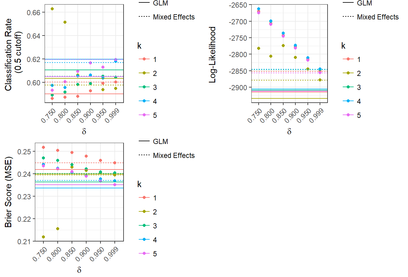
Figure 3.1: Model Evaluation

From Figure 3.1, we can observe that all of the models have different strengths. The discounted likelihood model with the smallest value of \(\delta\) consistently has the highest likelihood. However, it does not test as well as the other models in areas of out-of-sample classification rate and Brier score. This suggests that models with smaller values of \(\delta\), where the likelihood of an observed shot is more heavily influenced by shots closer to it, may overfit the model to the training data. The generalized linear models perform best in Brier score, but worst in log-likelihood. The hierarchical models are about the same as the GLMs, but they have a better log-likelihood performance. A model that balances the trade-off between predictive accuracy and likelihood is a discounted likelihood model with \(\delta\) = 0.850.

In addition, we can see that the overall variation in model performance is small. For example, most of the out-of-sample classification rates fall between 0.58 and 0.62. This is within the 95% confidence interval for a random binomial proportion of 0.6 using a sample size of 40 (because there are 8 different models and 5 train-test splits for each model), which is (0.5225, 0.6775). Therefore, the evidence that the models without discounting predict better than the ones with discounting is not particularly strong.

For the discounted likelihood model with \(\delta\) = 0.850, we build calibration plots to assess how well the estimated probabilities fit the actual proportions. To make these plots, we divide the predicted probabilities into 20 equally-sized bins, then plot these bins on the x-axis with the proportions of the actual outcomes within the bins on the y-axis. The horizontal bars represent the bin width, and the vertical bars represent a 95% confidence interval of the proportions. The red line of slope 1 represents equality between the bin medians and the empirical probabilities within the bins. In Figure 3.2, we present these plots for a full training set and a testing set.

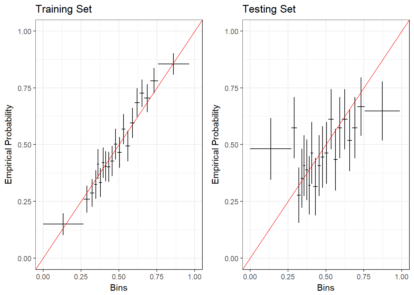
Figure 3.2: Calibration Plots for Discounted Likelihood Model, \(\delta\) = 0.850

We can see that the confidence intervals on the training set all cross the line of slope 1, which shows that the model output reliably fits the probabilities. In the testing set, however, the predictions only cross this line between about 0.3 and 0.75. In addition, the widths of the bins on the edges show that the model is not likely to predict values close to 0 or 1.

3.2 Results from Model with \(\delta\) = 0.850

To illustrate results from the discounted likelihood model with \(\delta\) = 0.850, we replicate the plots in Figures 2.5 and 2.6. The results are shown in Figure 3.3.

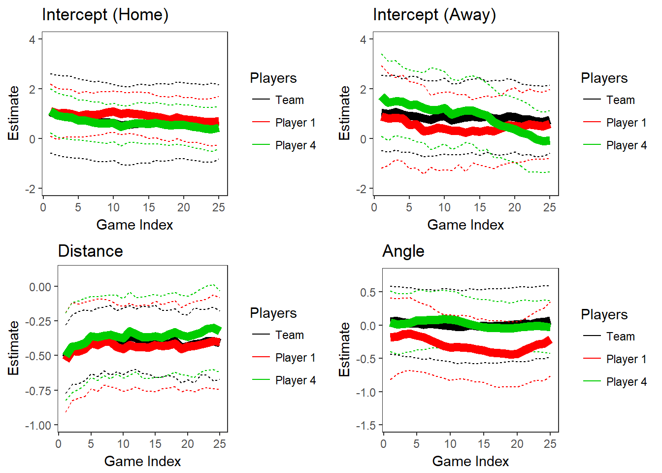
Figure 3.3: Parameters for Two Players and Population over Time, \(\delta\) = 0.850

Figure 3.3 has smoother changes over time than in Figure 2.5, where \(\delta\) = 0.750, which could indicate that there is less overfitting. One surprising result from this model is how the distance parameters slightly increase over time, and the intercepts slightly decrease. This could be a result of team shot selection evolving throughout the season, or just a coincidental signal.

3.3 Conclusion

The evaluations of the models show that there is some weak evidence for time-dependency in shooting success rate in this dataset of player-tracking data from the Duke Men’s Basketball team. Allowing predictors of shot success to shift based on recent success does not significantly improve the predictive accuracy of a model. However, we do see a systematic improvement in likelihood for smaller discount factors (i.e., more emphasis on recent shots, and therefore support of “streakiness”). Weaknesses of the discounting model include a smaller sample size and poorer out-of-sample prediction. Takeaways that we observed in other models include the fact that the angle of the shot only matters for certain players, and it is not a significant predictor of shot success between all players. Also, the effects of home-court advantage are not strong in this dataset, possibly due to the fact that most of the games away from home are missing.

To account for possible unexplained variation between seasons, and for variation introduced from having such a small population of road games, I repeated this analysis on a subset of the data that only consisted of shots from available games in one season (25 games), and shots from all home games (82 games). The results were similar, except for increased uncertainty due to smaller sample sizes. The model evaluation plots show similar patterns to the ones in Figure 3.1, and they are presented in Appendix B.

3.4 Future Goals

Future goals for this research are to build a better-fitting model to predict basketball shots using more advanced factors that can be approximated from the dataset. Possibilities for this include reparametrizing the location of a shot using categories (e.g., corner three-point shots, heaves from half-court) using the distance of the nearest defender as a proxy for defense quality, or using the amount of time a player has played without a substitution or timeout to approximate fatigue. In addition, we make the unrealistic assumption that every player exhibits the same amount of shooting streakiness with our discounted likelihood models. We could improve upon this assumption in the discounted likelihood models by adding a random effect on \(\delta\), to allow it to vary by player.