Chapter 2 Models & Analysis
2.1 Description of Models
For our models, we consider the shot location, a home court indicator, the shooter’s identity, and his shooting outcomes in nearby games as factors that can affect a shot’s outcome. We use the Just Another Gibbs Sampler library in R (R2jags) to build these models. Each one is based on a logistic regression model that provides the posterior distribution of the shot location parameters (distance and angle) and an additional intercept to capture the influence of home-court advantage. The models do not account for covariance between these predictors. We expand upon this model by adding mixed effects and discounted likelihood models to control for shooter identity and between-game variability, respectively. In our Gibbs Samplers, we estimate the posterior distributions using 10,000 simulations and a burn-in of 500. Our prior distributions are constructed from the corresponding maximum likelihood estimates for the first four games in the dataset, and we initialize our Monte Carlo Markov Chains using values of 0 for all means, and 1 for all variances. The R2jags code used to build these models can be found in Appendix A.
2.1.1 Generalized Linear Model
We start with a logistic regression model for each shot attempt \(i\):
\[ \text{logit}(p_{i}) = \beta_{\text{int}} + x_{\text{r,i}}\beta_{\text{r}} + x_{\theta,\text{i}}\beta_{\theta} + x_{\text{H,i}}\beta_{\text{H}}. \]
In this model, the \(x\) refers to the data, and the \(\beta\)s are the parameters from the model. The subscripts \(\textit{int}\), \(\textit{r}\), \(\theta\), and \(\textit{H}\) respectively refer to the intercept, the log-distance of the shot, the angle of the shot, and whether shot was taken on Duke’s home court or another gym. This fourth \(\beta\) accounts for the possibility of “home-court advantage”, which can affect shot outcomes.
2.1.2 Hierarchical Generalized Linear Model
Our second model is a hierarchical model, with random effects on the \(\textit{j}\) players in the dataset. These random effects occur for each of the four parameters of interest—the intercept, the distance effect, the angle effect, and the home effect. Each individual player’s parameter values are sampled from a Normal distribution centered at the population values. A benefit of this type of model is that the parameters for players with few shot attempts are shrunk towards the population means. The model has the form below for each player \(j\) and shot attempt \(i\):
\[ \text{logit}(p_{\text{ji}}) = \beta_{\text{int, j}} + x_{\text{r,ji}}\beta_{\text{r, j}} + x_{\theta,\text{ji}}\beta_{\theta, \text{j}} + x_{\text{H, ji}}\beta_{\text{H, j}}, \] \[ \beta_{\text{int, j}} \sim N(\beta_{\text{int}}, \tau^2_{\text{int}}), \] \[ \beta_{\text{r, j}} \sim N(\beta_{\text{r}}, \tau^2_{\text{r}}), \] \[ \beta_{\theta, j} \sim N(\beta_{\theta}, \tau^2_{\theta}), \] \[ \beta_{\text{H, j}} \sim N(\beta_{\text{H}}, \tau^2_{\text{H}}). \]
2.1.3 Discounted Likelihood Hierarchical Model
In the discounted likelihood models, the likelihood function for all model parameters at a given time is more heavily influenced by the observations close to that specific time point than the observations far away from it. We measure the “distance” between observations by the number of games between them; a shot attempt that occurs in the next or the preceding game will influence the likelihood function for the parameters “anchored” at that game more than a shot that occurs two games away. We chose to analyze time-dependency in the data using a discounted likelihood model instead of a full dynamic model because a discounted likelihood model would have fewer complications in the context of a hierarchical model. The methodology behind our discounted likelihood model relates closely to Bayesian dynamic modeling that uses power discounting to reduce the effect of data that occurs further in the past. We begin defining this model with the concept of forward filtering. This is implied by a power-discount Bayesian time series model (Smith, 1979) that uses a “discounted” Bayes Theorem in which the posterior disitribution of the model parameters at any chosen time \(t\) is proportional to the product of the prior, \(p(\Theta)\), and the discount likelihood function, which has the form

\[ p_t(X_{1:t}|\Theta) = p_t(X_{1:t-1}|\Theta)p(X_t|\Theta), \]
where
\[ p_t(X_{1:t-1}|\Theta) \propto p(X_{1} |\Theta)^{\delta^{t-1}}... p(X_{t-2}|\Theta)^{\delta^{2}} p(X_{t-1}|\Theta)^{\delta} \]
for some discount factor \(0 < \delta < 1\), typically closer to 1 to allow for the discounting of past data without omitting its information content.
This equation shows that as distance increases backward in time, the effect on the likelihood function—and hence on the resulting posterior for \(\Theta\) at our current time \(t\)—decreases. The corresponding discount likelihood for \(\Theta\) at time \(t\) given both past and future data up to a time \(T > t\) has a similar form, but with two-sided discounting. This relates to dynamic models with time-varying parameters, which apply backwards updating to update their posteriors. The form of the two-sided likelihood function of \(\Theta\) at a chosen time \(t\) is:
\[ p_t(X_{1:T}|\Theta) = p_t(X_{1:t-1}|\Theta) p(X_{t}|\Theta) p_t(X_{t+1:T}|\Theta), \]
where the past data component \(p_t(X_{1:t-1}|\Theta)\) is the same as above, and the future data component is:
\[ p_t(X_{t+1:T}|\Theta) \propto p(X_{t+1}|\Theta)^{\delta} p(X_{t+2}|\Theta)^{\delta^2}... p(X_{T}|\Theta)^{\delta^{T-t}}. \]
Specifically for our model, given an observed shot \(\textit{i}\) in game \(g\), attempted by player \(\textit{j}\), we apply the above reasoning to discount the likelihood of a made shot in the hierarchical model. First we begin with a hierarchical logistic regression model:
\[ \text{logit}(p_{\text{gji}}) = \beta_{\text{int, gj}} + x_{\text{r,gji}}\beta_{\text{r, gj}} + x_{\theta,\text{gji}}\beta_{\theta, \text{gj}} + x_{\text{H, gji}}\beta_{\text{H, gj}}, \] \[ \beta_{\text{int, j}} \sim N(\beta_{\text{int}}, \tau^2_{\text{int}}), \] \[ \beta_{\text{r, j}} \sim N(\beta_{\text{r}}, \tau^2_{\text{r}}), \] \[ \beta_{\theta, j} \sim N(\beta_{\theta}, \tau^2_{\theta}), \] \[ \beta_{\text{H, j}} \sim N(\beta_{\text{H}}, \tau^2_{\text{H}}). \]
Without discounting, the likelihood term controbuted from a shot’s outcome, \(\text{y}_\text{gji}\), that is attempted by player \(\textit{j}\) in game \(\textit{g}\), is:
\[ L_\text{gj}(\Theta) = \prod_{\text{i}=1}^{\text{n}_\text{gj}}{ p(\text{y}_{\text{gji}} | \Theta) } \propto \prod_{\text{i}=1}^{\text{n}_\text{gj}}{ p_\text{gji}^{\text{y}_\text{gji}} (1 - p_\text{gji})^{1-\text{y}_\text{gji}} }. \]
When we apply the exponential discounting to the outcomes like so:
\[ \pi_{\text{gji}} = \left( p_\text{gji}^{\text{y}_\text{gji}} (1 - p_\text{gji})^{1-\text{y}_\text{gji}} \right) ^{\delta^{|g-g_0|}}, \]
our likelihood becomes:
\[ \Lambda_{\text{gj}}(\Theta) = \prod_{\text{i}=1}^{\text{n}_\text{gj}} \pi_{\text{gji}}, \]
where \({g}\) is the game index of the current shot \(\textit{i}\), and \(g_0\) is a fixed game index, which we refer to as the “anchor game”.
In this model, \(p\) represents the binomial probability, and \(\pi\) is the discounted probability. Both of these quantities are probabilities that are bounded in the interval [0,1]. Similarly, \(L\) is the likelihood and \(\Lambda\) is the discounted likelihood. The contribution of shot outcomes from games \(g\) that are more distant from the anchor game \(g_0\) are more heavily discounted, and the discounting increases for smaller values of \(\delta\). In a model with \(\delta\) = 0, only shots taken in the same game as shot \(i\) can contribute to the likelihood, while \(\delta\) = 1 is equivalent to a model with no discounting. If models with larger values of \(\delta\) best fit the data, this suggests that shooting success is consistent throughout a career. If smaller values of \(\delta\) are more likely in the data, however, then we can assume there is a substantial amount of time variation, or “streakiness”, in the data on the game level. Figure 2.1 illustrates how the exponential weight on the likelihood depends on the selected value of \(\delta\) and the distance from the anchor game (\(g - g_0\)).

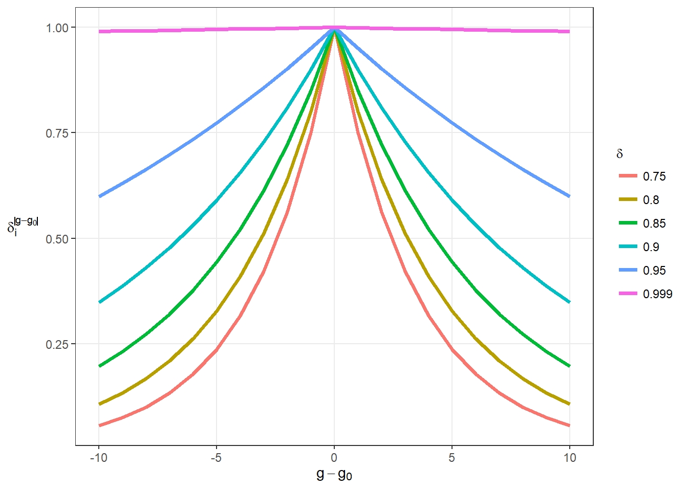
Figure 2.1: Illustration of Discounted Weighting
This model specification is specific to the chosen anchor game \(g_0\), so that the resulting posterior distribution for all model parameters is indexed by \(g_0\) and represents inferences “local” to that game. Repeating the analysis across all games as anchors results in a sequence of posteriors, where their differences reflect time variation. As a result, we refit the model using MCMC for each combination of game index and \(\delta\), which involves substantial computation.

To build these discounted likelihood models in the R2jags library, we apply the “ones trick”. This technique allows us to use a sampling distribution that does not exist in the library by modifying a common distribution—in this case, the Binomial. The probability \(p\) is estimated in the same way as the Bayesian hierarchical model. We discount this probability to estimate \(\pi\), and then we specify that it comes from Binomial data that consists only of ones; this is equivalent to sampling from a distribution with discounted outcomes. In the code excerpt below, result and prob are the binomial outcomes and probabilities, while y represents the “trick” outcomes (a vector of 1s), and pi is the discounted probability.

    for(i in 1:N){

      # delta = discount rate for game g relative to anchor game g0
      wt[i] <- delta^abs(games[i]-g0)

      # player-level random effects
      logit(prob[i]) <- beta_int[player[i]]*int[i] +
                        beta_home[player[i]]*home[i] +
                        beta_r[player[i]]*logr[i] +
                        beta_theta[player[i]]*theta[i]

      # likelihood function
      p1[i] <- prob[i]^result[i]
      p2[i] <- (1-prob[i])^(1-result[i])

      # discounted likelihood function
      pi[i] <- (p1[i] * p2[i])^wt[i]

      # defines correct discounted likelihood function
      y[i] ~ dbern(pi[i])

    }

    # Priors
    for(j in 1:M){
      beta_int[j] ~ dnorm(beta_int0,tau_int)
      beta_home[j] ~ dnorm(beta_home0, tau_int)
      beta_r[j] ~ dnorm(beta_r0,tau_r)
      beta_theta[j] ~ dnorm(beta_theta0,tau_theta)
    }
See Appendix A.3 for the full R code.
2.2 Analysis
2.2.1 Generalized Linear Model
In our generalized linear model, we only look at shot location and the home court indicator as predictors of shot outcome. This is a logistic regression model where the intercepts correspond to the log-odds of making a shot when the angle is zero (the middle of the court) and the log-distance is zero (one foot away from the rim). To illustrate these effects for individual players, we simply subset the dataset to include only shots attempted by that player before running the Gibbs Sampler. In Figure 2.2, The 95% credible intervals of the posterior parameters are reported for the same four players that were introduced in Figure 1.2.

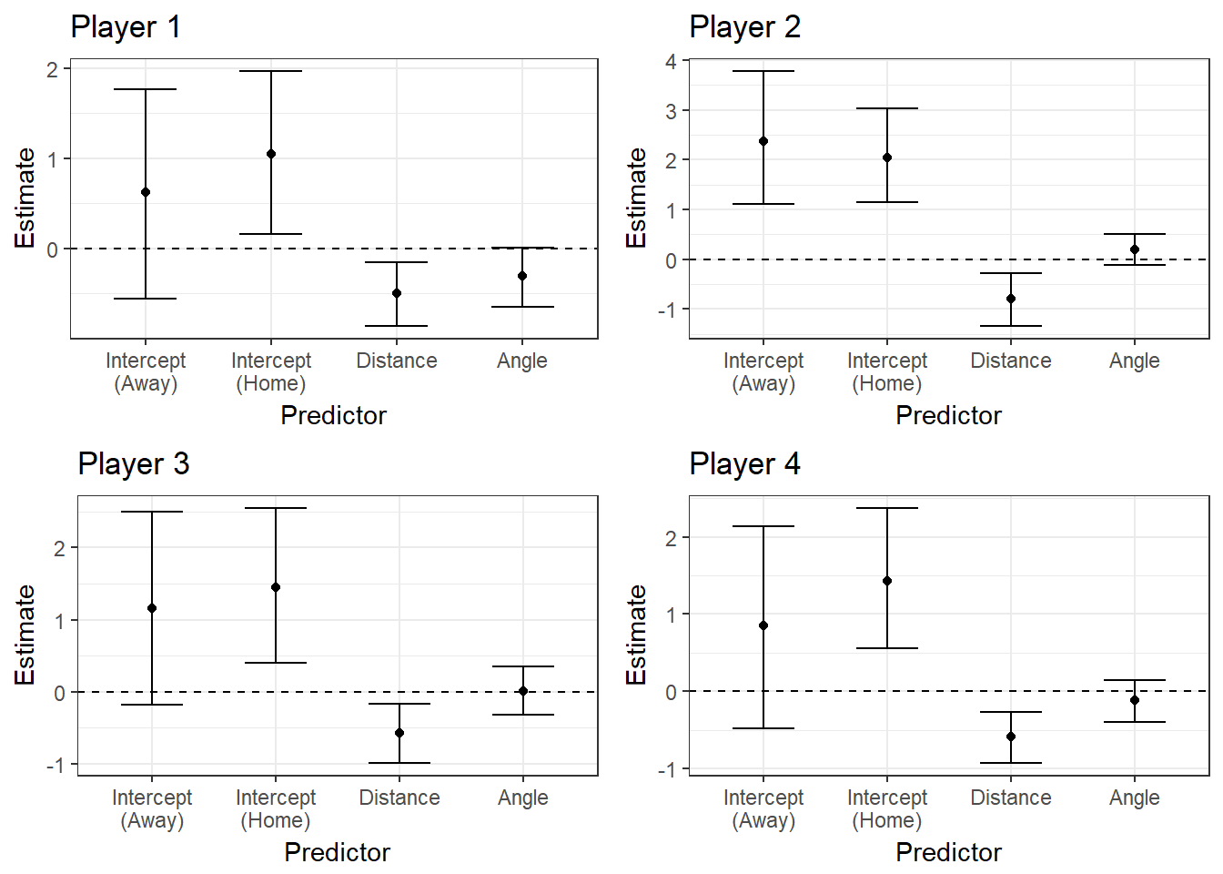
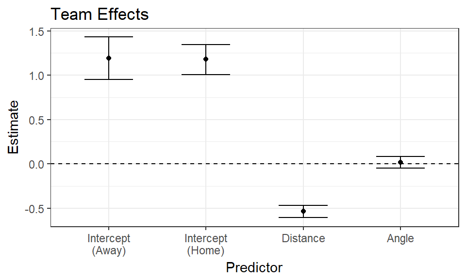
Figure 2.2: GLM Posterior Distributions for Four Players
From these plots, we see that the team-wide 95% credible interval of the angle effect is centered at zero, and it is therefore probably not predictive of a made shot. The average distance effect shows us that the log-odds of a made shot decrease by \(\beta_r =\) 0.5372 as the log-distance increases by one unit and the other predictors remain constant. This effect is translated to the probability scale using the expression
\[ \frac{\text{e}^{\beta_r}}{1 + \text{e}^{\beta_r}}, \]
which equals 0.3689.
We also see that the 95% credible interval on the effect of distance is completely negative, which follows the intuitive idea that the probability of a made shot significantly decreases as distance from the basket increases. The intercepts show us that there is not a substantial difference in baseline shooting performance between home games and away games. The interval for away games is wider because there are fewer of them in the dataset.
2.2.2 Hierarchical Generalized Linear Model
To make the hierarchical model, we add random effects that allow the parameters to vary for each player in the dataset. For every linear covariate in the model, we model player-specific effects as sampled from a Normal distribution roughly centered at the covariate’s population mean. We present the results in Figure 2.3 by comparing the effects of the four high-usage players of interest to the population density of each covariate.
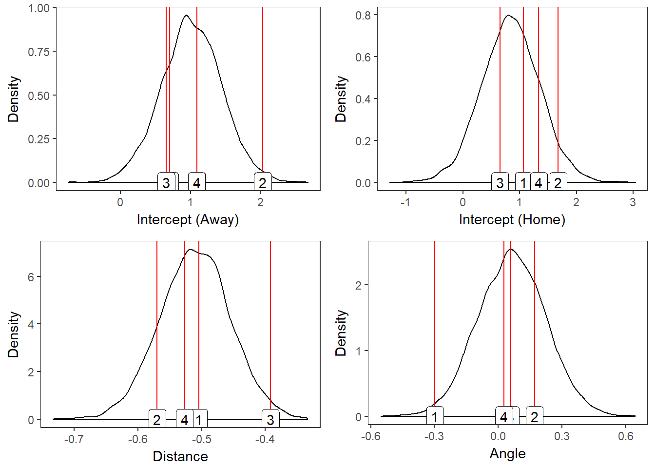
Figure 2.3: Population Distribution with Four Player Effects
The plots in Figure 2.3 show us that Player 2 excels at scoring under baseline conditions (close to the basket), but he has a steeper-than-average drop in his odds of scoring as his distance from the basket increases. We can also see that Player 1 strongly increases his odds of scoring when his angle is negative, which corresponds to the left side of the basket, while the other three players’ effects are all close to zero.
In Figure 2.4, we present contour plots showing the players’ expected field goal percentages at all locations on the half of the court where they are shooting. We compute these from the fitted probabilities of shot success from the hierarchical model. This plot confirms that Player 1 is more effective on the left side of the basket than the others. Other takeaways that were not noticeable in Figure 2.3 are that Player 2 has the darkest overall contour plot, which suggests that he has the highest overall probability of scoring, and that Player 4 has lightest plot, suggesting he is the least reliable scorer among these four players.
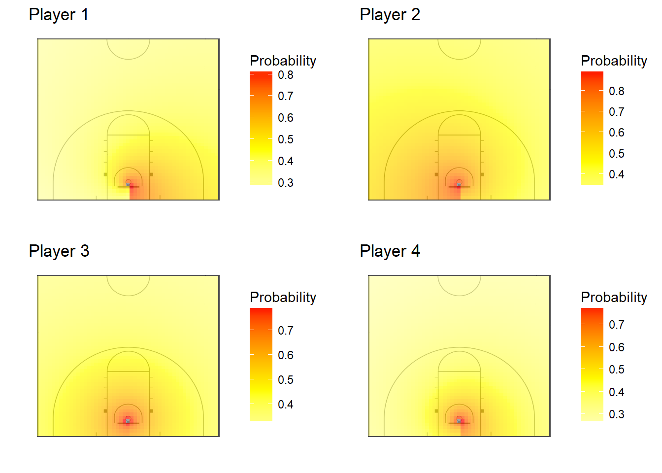
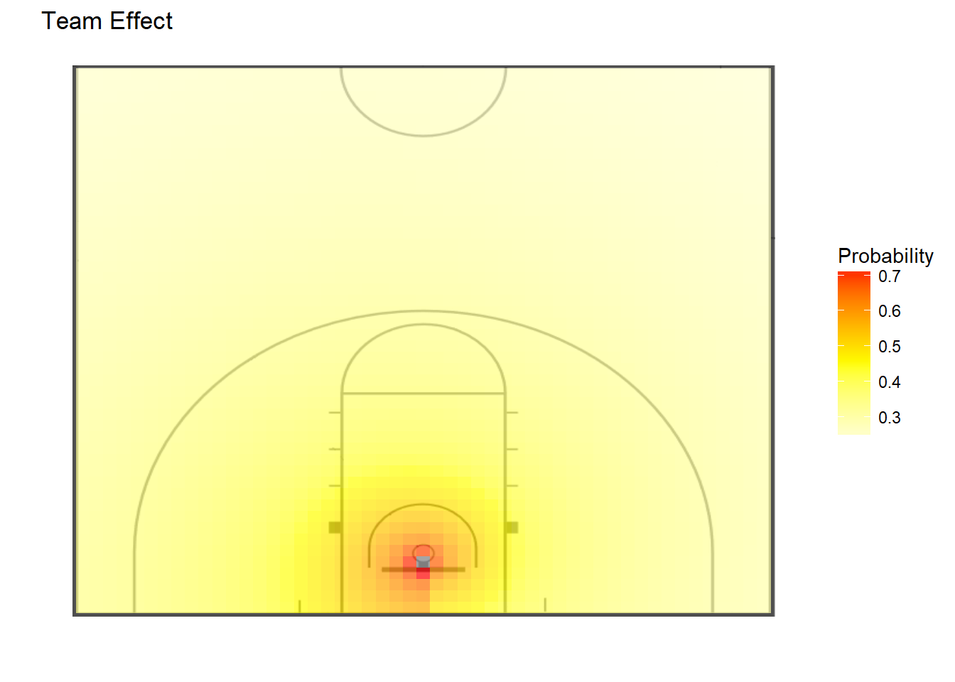
Figure 2.4: Contour Plots for Four Players and Population of Players
2.2.3 Discounted Likelihood Hierarchical Model
The values of \(\delta\) that we use to fit the discounted likelihood models are 0.750, 0.800, 0.850, 0.900, 0.950, and 0.999. For each of these values, we refit the model to generate a full MCMC sample from the posterior, using every game as the anchor game \(g_0\). We calculate predictions and fitted values for a particular shot in game \(g\) using the posterior median of the MCMC chain where \(g\) is the anchor game \(g_0\). The plots in Figure 2.5 and 2.6 show how the posterior parameter distributions (95% credible intervals) change over the course of one season on the team level and for two players (the other two players are not shown here because they did not play during this season). Figure 2.5 illustrates the results for our smallest value of \(\delta\), 0.750, and 2.6 shows them for our largest value of \(\delta\), 0.999.
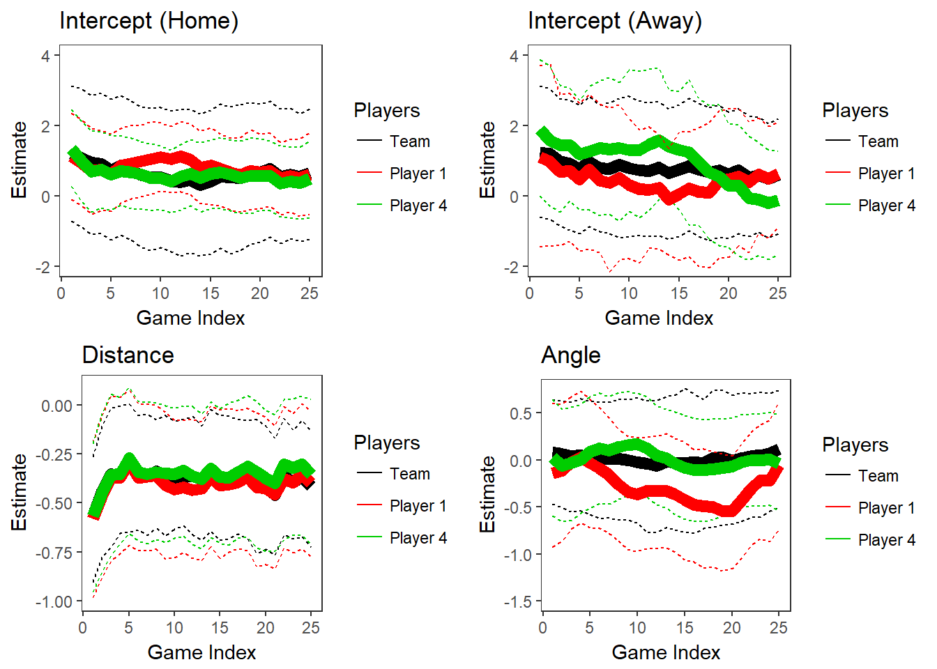
Figure 2.5: Parameters for Two Players and Population over Time, \(\delta\) = 0.750
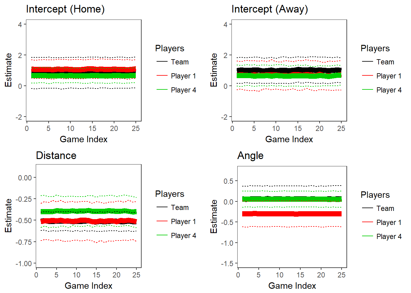
Figure 2.6: Parameters for Two Players and Population over Time, \(\delta\) = 0.999
These plots illustrate how smaller values of \(\delta\) allow for more variation in the posteriors over time. Another observation from this plot is that the credible intervals are wider when \(\delta\) is smaller. Between the two plots of the home game intercepts, we can see that the 95% credible in the first game when \(\delta\) = 0.750 ranges from about -1 to 3, while the corresponding interval in the plot where \(\delta\) = 0.999 ranges from about 0 to 2. The uncertainty in the posteriors increases as the discounting parameter \(\delta\) decreases because a smaller \(\delta\) corresponds to fewer observations contributing to the likelihood.