Chapter 1 Data
1.1 Description of Dataset
The data for this analysis comes from SportVU, a player-tracking system from STATS, LLC. that provides precise coordinates for all ten players and the ball at a rate of 25 times per second. The Duke University Men’s Basketball team permitted us to use their SportVU data from the 2014 to 2017 basketball seasons for this project. Since the ability to record this data depends on specialized tracking cameras, Duke does not have this data for every game they play—only home games, and a few road games in arenas that had the technology installed. Therefore, there is a substantial amount of missing data between games. More specifically, between the 2014 and 2017 seasons, the Duke Men’s Basketball team played 147 games; this dataset contains 94 games, with 82 at Duke and 12 at other arenas.
For our analysis, we use the following files for each game:
- Final Sequence Play-by-Play Optical:
This dataset comes in an a semi-structured Extensible Markup Language (XML) file, where there is a unique element for each “event” (an event is a basketball action such as a dribble, pass, shot, foul, etc.). Each event element has attributes describing the type of event, the time of the event, and the player who completed the action. We use these files to uncover when a shot is attempted in a game, who attempted the shot, and the result of the shot attempt.
- Final Sequence Optical:
These XML files contain the locations of all ten players and the ball during precise time intervals within the game (25 times per second). Each time unit has a unique element, and these elements have attributes describing the locations. We merge this with the Final Sequence Play-by-Play Optical data on the time attribute to obtain the shooter’s location at the moment of a shot attempt.
1.2 Data Cleaning
Steps taken to clean the merged shooter IDs with shot locations include translating the locations to a half-court setting (the teams switch sides of the court halfway through every game, which means that we have to flip the coordinates across the middle of the court for about half of the shots in every game), converting the x-y coordinates to polar coordinates (in the units of feet and radians), and adding an indicator for home games. We only use the shots that Duke players attempt, because there is an inadequate amount of data for players on other teams—no opposing players appear in more than 5 games. The final dataset contains 5,467 observations from 31 shooters over 94 games. A summary of the cleaned dataset is in Table 1.1:
| Name | Type | Values | Extra Details |
|---|---|---|---|
| season | categorical | {2014, …, 2017} | |
| gameid | categorical | NA | 94 unique values |
| time | continuous | NA | 13-digit timestamp in milliseconds |
| globalplayerid | categorical | NA | 31 unique values |
| r | continuous | [0, \(\infty\)) | Distance of shot from basket (feet) |
| theta | continuous | [-\(\pi\), \(\pi\)] | Angle of shot (radians) |
| home | categorical | {0,1} | 1 if shot occured in a home game |
| result | categorical | {0,1} | 1 if shot was made (response) |
A small subset of the cleaned data is displayed below in Table 1.2:
| season | gameid | time | globalplayerid | r | theta | home | result |
|---|---|---|---|---|---|---|---|
| 2014 | 201401070173 | 1389141733839 | 603106 | 4.2076 | 1.0746 | 1 | 1 |
| 2014 | 201401070173 | 1389141844712 | 601140 | 16.6537 | 1.2973 | 1 | 0 |
| 2014 | 201401070173 | 1389143172185 | 696289 | 18.7901 | -0.0581 | 1 | 1 |
| 2014 | 201401070173 | 1389143196303 | 601140 | 23.4629 | 0.9539 | 1 | 1 |
| 2014 | 201401070173 | 1389143220261 | 756880 | 6.5365 | 0.0696 | 1 | 0 |
Figure 1.1 shows the locations of all the shots in the dataset, translating the locations to one half of the court, and excluding heaves from beyond half court. The variable \(\theta\) has a range of \(2\pi\) radians, but this plot shows that most of the attempts occur within the interval (-\(\frac{\pi}{2}\), \(\frac{\pi}{2}\)). This figure also shows the bimodal distribution of shot distance over all players.
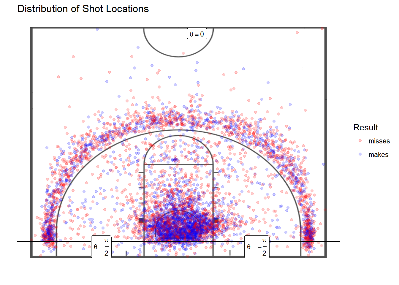
Figure 1.1: Locations and Results of All Shots
1.3 Exploratory Data Analysis
The exploratory data analysis plots in Figure 1.2 examine how consistent the probability of a made shot is, using a loess smooth curve on the binary outcomes. We present these smoothed plots for four high-usage basketball players at Duke University between the 2014 and 2017 seasons. Each plot represents a single player’s ordered shooting outcomes for a single season. These plots do not account for the amount of time in between shots, but simply shot order and outcome.
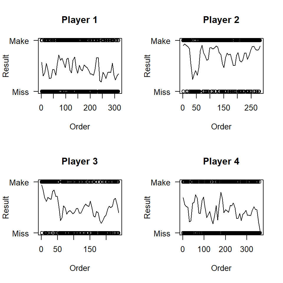
Figure 1.2: Moving Average of Shot Success Rate
We can see that the players vary in the consistency of their made shots, since they all contain spikes and trends. For example, Player 3 initially has a very high success rate, which quickly falls to the middle after about 30 shot attempts, and the Player 2 has a noticeable upward trend in shot success beginning around shot number 150.
We investigate the shooting outcomes using Bayesian models, and present the results in the next chapter.