Chapter 5 Results
Both numerically and graphically, the student projects inspected in this study using the tidyverse syntax scored higher on all three of the developed metrics. Tidyverse projects were much more prevalent in the upper levels of the three variables, and their means and standard deviations significantly differed as well.
5.1 Creativity Metric
Despite there being only 82 base R projects recorded to the 123 tidyverse projects, there more base R projects scored a 0 or 1 on the creativity metric than those using the tidyverse syntax. Overall, there was a single project that scored a perfect 4 out of the 193 projects, and the majority of the projects scored a 1 or 2 in the creativity metric.
However, within the tidyverse projects, more than half (56.1 percent) registered at least a 2 on creativity, compared to just 20.7 percent of base R projects.
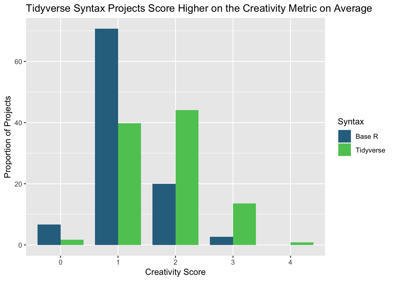
The average creativity scores and corresponding standard deviations for projects utilizing the two syntaxes are available below as well:
| Syntax | Mean | SD |
|---|---|---|
| Base R | 1.1 | 0.6 |
| Tidyverse | 1.7 | 0.8 |
| Syntax | Mean | Standard Deviation |
|---|---|---|
| Base R | 1.1 | 0.6 |
| Tidyverse | 1.7 | 0.8 |
FOR MINE: Which table should I use? One has SD as Standard Deviation
When dissected by semester, the creativity score distributions did not notably vary for sections taught in base R. However, two sections—both employed the tidyverse syntax-from the Spring 2016 semester fared significantly better by their score breakdown than the other tidyverse courses. Without those two semesters of tidyverse projects, the rest of the tidyverse projects still boasted a higher score distribution than those of base R. Still, this discrepancy may be due to advanced instruction from the teaching assistants that encouraged groups to satisfy the requirements for higher creativty scores. Rhe following subsections will contain a comparison of base R and tidyverse student projects for each of the four variables combined to form the creativity metric, as well as potential reasons for the outcomes.
5.1.1 Creation of New Variable(s)
Out of the four variables that form the creativity metric, the starkest difference between projects employing the two syntaxes was within the creation of new variable(s) covariate. Nearly half of all final projects using the tidyverse syntax featured a creation of a new variable, whereas less than a quarter of base R projects did.
| tidyverse | create_new_var | n | proportion |
|---|---|---|---|
| base R | yes | 18 | 24.0% |
| tidyverse | yes | 59 | 50.0% |
This difference may be due to the ease in utilizing the tidyverse’s mutate() function, which allows users to create new variables using a single command. In base R, students are instructed to use $ notation, which may be harder to grasp due to issues with variable selection with $ and its usage in other base R tasks outside of creating new variables.
5.1.2 Transformation of Existing Variables
While more than 75 project groups created new variables, far less opted to mutate existing ones in the movies dataset. Because the counts for both base R and tidyverse projects that satisfied this variable were lower, the resulting proportions were also much smaller. Regardless, there were more projects using the tidyverse syntax that mutated existing variables.
| tidyverse | change_var | n | prop |
|---|---|---|---|
| base R | yes | 2 | 2.7% |
| tidyverse | yes | 9 | 7.6% |
The difference in proportions was not nearly as significant as it was for the creation of new variables and only differed marginally. This limited difference can be attributed to two factors. First, with the option to create their own variables, groups may not find transforming existing variables as appealing. Second, the mechanism to do so does not differ dramatically between the two syntaxes. For comparison, an example of changing an existing studio variable to “Warner Bros. Studios” or “Other” is listed in both Base R and the tidyverse:
Base R: movies$studio <- if_else(movies$studio == "Warner Bros. Pictures", "Warner Bros. Pictures", "Other")
Tidyverse: movies <- movies %>% mutate(studio = (if_else(studio == "Warner Bros. Pictures", "Warner Bros. Pictures", "Other"))
5.1.3 Existence of Subgroup Analysis
Out of all the covariates forming the creativity metric, the subgroup analysis was the most popular one satisfied for both base R and tidyverse projects. 93.5 percent of tidyverse projects performed a type of subgroup analysis, while more than 3/4 of base R projects did.
| tidyverse | sub_analysis | n | prop |
|---|---|---|---|
| base R | yes | 65 | 86.7% |
| tidyverse | yes | 115 | 97.5% |
The popularity of this aspect within group projects may be explained by the copious ways student groups could perform a subgroup analysis. However, subgroup analyses may be easier to perform in the tidyverse due to the presence of the group_by() command, which is usually one of the most popular functions for beginning R users in the tidyverse. In contrast, base R’s by() function is not nearly as well-known.
5.1.4 Use of a Data Subset for Project’s Entirety
The use of a subset of the provided movies dataset for the entire final project was also significantly more popular amongst tidyverse projects, as more than 15 percent of student projects using the tidyverse satisfied a score of a one for this covariate, compared to less than 5 percent of all base R projects.
| tidyverse | sub_data | n | prop |
|---|---|---|---|
| base R | yes | 4 | 5.3% |
| tidyverse | yes | 20 | 16.9% |
Since there is little difference between the tidyverse’s filter() and base R’s subset() functions, this discrepancy might not have a distinct explanation. Perhaps, though, student groups using the tidyverse may have been more encouraged to utilize data subsets throughout their projects more often than those in base R because other creativity aspects were performed more frequently in tidyverse projects, so those groups may have gained additional insights that led them to use data subsets that base R project groups did not discover.
5.2 Depth Metric
Although the depth metrics scores between final projects that employed base R syntax compared to those using the tidyverse do not have a similar discrepancy as the one for the creativity score, there is still a considerable difference in the depth metric distributions between projects of the two syntaxes.
48.8 percent of the projects using the tidyverse syntax scored a perfect 2 in the depth metric compared to 34.1 percent of base R projects, while the extreme majority of base R projects scored a 0 or 1 in the depth metric. Overall, most projects scored a one.
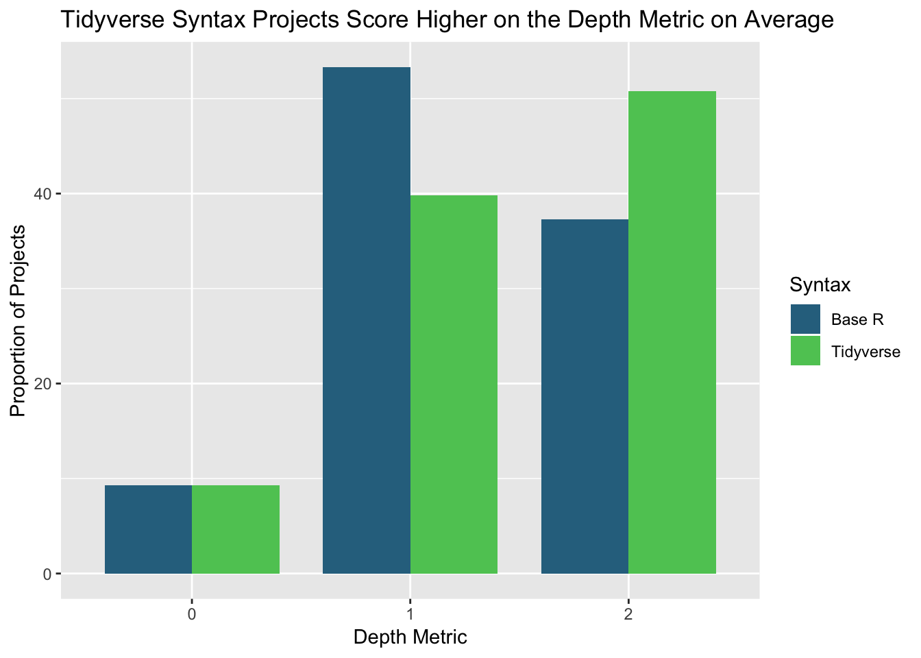
The average depth scores and corresponding standard deviations for projects utilizing the two syntaxes are available below as well:
| Syntax | Mean | SD |
|---|---|---|
| Base R | 1.2 | 0.7 |
| Tidyverse | 1.4 | 0.7 |
FOR MINE: Which table should I use? One has SD as Standard Deviation
| Syntax | Mean | Standard Deviation |
|---|---|---|
| Base R | 1.2 | 0.7 |
| Tidyverse | 1.4 | 0.7 |
The results of the depth metric may be due to the simplicity of command chains in the tidyverse that make the project easier to code for beginners in R.
Upon inspection by class section, the depth score distributions were largely similar, sans one of the Spring 2016 sections. Similar to how projects from this section performed on the creativity metric, they scored much higher on average in the depth category than projects from the other classes. The following subsections will contain a comparison of base R and tidyverse student projects for the two variables combined to form the depth metric.
5.2.1 Consistent Theme
Within the theme metric, the variable tracking the presence of a consistent theme showcased a larger difference in proportions between base R and tidyverse student projects. Compared to base R projects, where 57.3 percent boasted a consistent theme, 71.5 percent of all tidyverse projects maintained uniformity theme-wise.
| tidyverse | eda_theme | n | prop |
|---|---|---|---|
| base R | yes | 47 | 62.7% |
| tidyverse | yes | 88 | 74.6% |
The difference in proportions may potentially be attributed to the prevalence of select() and filter() within the tidyverse syntax, which allows users to choose specific columns within a data that satisfy a certain criteria, compared to base R, when student groups commonly utilized square brackets to delineate those same criteria.
5.2.2 Presence of Relevant Data
Proportions for the presence of relevant data covariate were very similar, with just a 4.4 percent difference in proportions (64.2 for tidyverse compared to 59.8 for base R projects) between projects using the two syntaxes.
| tidyverse | rel_data | n | prop |
|---|---|---|---|
| base R | yes | 49 | 65.3% |
| tidyverse | yes | 79 | 66.9% |
The presence of relevant supporting data should not be greatly impacted by the particular coding syntax student groups employed, which may explain the small difference in proportions for this variable.
5.3 Multivariate Visualization Metric
Between projects using the two different syntaxes, the most significant difference in any of the three metrics occurred within the multivariate visualization metric, where just one final project in base R even displayed a plot containing at least three different variables. The majority of all projects did not include multivariate visualizations, but projects using the tidyverse syntax were more popular within higher scores of the metric in general, with 13 percent scoring a perfect 2. No projects in base R reached the same score.
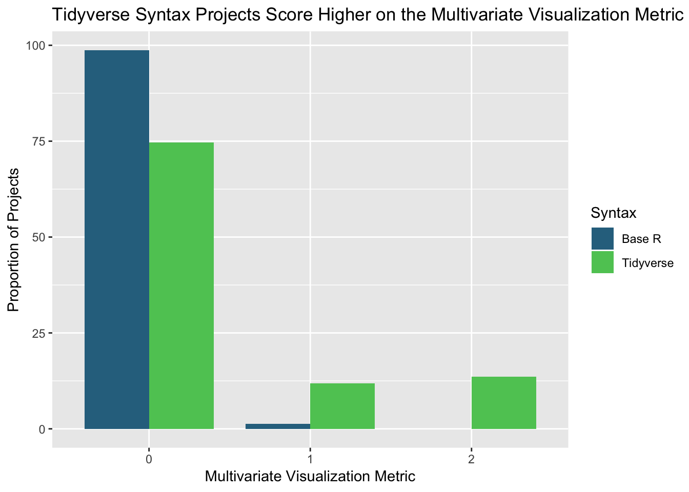
The average multivariate visualization scores and corresponding standard deviations for projects utilizing the two syntaxes are available below as well. Although the statistics do not represent the difference in the metric between projects of the two syntaxes, there is still a distinct divide.
| Syntax | Mean | SD |
|---|---|---|
| Base R | 0.0 | 0.1 |
| Tidyverse | 0.4 | 0.7 |
FOR MINE: Which table should I use? One has SD as Standard Deviation
| Syntax | Mean | Standard Deviation |
|---|---|---|
| Base R | 0.0 | 0.1 |
| Tidyverse | 0.4 | 0.7 |
Although we have observed a higher rate and score distribution of tidyverse projects, the trend is not consistent by semester. One of the Fall 2015 sections included 10 projects with a multivariate visualization score of at least a one, while the other did not contain a single project showcasing a multivariate plot. Similar to the reasoning stated in the Creativity section, this may be due to the emphasis and quality of instruction from the teaching assistants (which differ by class section) in regards to creating plots with at least three variables. The following subsections will contain a comparison of base R and tidyverse student projects for the two variables combined to form the multivariate visualization metric.
5.3.1 Presence of a Visualization with 3+ Variables
Only one project coded in solely base R displayed a visualization with at least three variables, compared to 30 tidyverse projects. Percentage-wise, too, the tidyverse projects were more likely to contain a multivariate visualization.
| tidyverse | viz_mult_make | n | prop |
|---|---|---|---|
| base R | yes | 1 | 1.3% |
| tidyverse | yes | 30 | 25.4% |
These results may be due to the differences in base R’s plot() function relative to the tidyverse’s ggplot(). Whereas plot() requires extra commands to add graphical aesthetics besides x- and y-variables, the aes() command embedded within ggplot() provides an easy platform for tidyverse users to employ other aesthetics besides just the x- and y-variables. For example, code is listed below that would satisfy a score of one when using the two syntaxes.
Base R:
movies.color <- rep("pink", length(movies$best_pic_nom)) movies.color[movies$best_pic_nom == "yes"] <- "blue" plot(audience_score ~ critics_score, col = movies.color, data = movies) legend(col = c("pink", "blue"))
Tidyverse:
ggplot(data = movies, aes(x = critics_score, y = audience_score, color = best_pic_nom)) + geom_point()
FOR MINE: This code is correct, right?
5.3.2 Interpretation of Multivariate Visualization
No student project using solely base R interpreted a multivariate plot, whereas 13 percent of projects utilizing the tidyverse did. Although the proportion satisfying a score of a 1 is not very high, more than half of tidyverse projects that formed a visualization with at least three variables (16 out of 30) contained sufficient intepretations of the outputs.
| tidyverse | viz_mult_interpret | n | prop |
|---|---|---|---|
| tidyverse | yes | 16 | 13.6% |
Theoretically, the difference in proportions between projects primarily using base R compared to the tidyverse should not drastically differ. However, since there were more tidyverse projects that contained multivariate plots, there was bound to be a difference in this covariate. In general, though, the plots should not deviate for interpretation, though some users may find comfort in viewing graphs provided by their most commonly-used syntax.