Chapter 2 Methodology

2.1 Identify Common Topics (Entire Corpus)

Seeing our corpus as a collection of review documents sharing some common topics, the task of extracting these topics can be framed as a topic modeling one. In particular, we use Latent Dirichlet Allocation (LDA) to extract hidden common topics in restaurant reviews.

2.1.1 Data Pre-processing

Standard text data cleaning procedure was followed for preprocessing the review corpus: all characters were transformed to lowercase, punctuations and numbers removed, stop words such as “I”, “me”, “she”, “is” also removed, whitespaces stripped and trimmed, and all words stemmed using Porter stemming algorithm.

2.1.1.1 N-Gramming

One optional yet particularly helpful preprocessing step was n-gramming. It captures word sequences that are better perceived or carry more meaningful information as a whole. For example, “White House” should be perceived as a single token instead of separately as “white” and “house”, and similarly “President of the United States” makes more sense as a whole. N-gramming is especially helpful when identifying word sequences that are specific to the context of the corpus. In the previous example, it would be crucial to identify “White House” and “President of the United States” as n-grams in a corpus consists of political blogs. In our case where the corpus is consists of restaurant reviews, we can expect to see context-specific n-grams such as “Mac ‘n Cheese” or “highly recommend”. We take the probabilistic approach for identifying these n-grams where the conditional probability of seeing the i-th word given the (i-1) th word. The n-gramming implementation code was modified based on the NGramming Processing Script (c) by Teague Henry. The procedure in this code is for each consecutive bigram sequence (\(word_1\), \(word_2\)):

Calculate \(n_{word_1}\) = number of occurrences of \(word_1\) in the corpus;
Calculate \(p_{word_2}\) = proportion of \(word_2\) in all non-\(word_1\) words in the corpus;
Calculate \(n_bigram\) = number of occurrences of bigram \(word_1\_word_2\) in the corpus;
Compute \({p-value} = P(N \geqslant n_{bigram})\) where N is the total number of consecutive co-occurrences of \(word_1\_word_2\) where \(N \sim Binomial(c_{word_1}, p_{word_2})\);
If \({p-value} < 0.01\), then we reject the null hypothesis that the co-occurrences happened by random and identify \(word_1\_word_2\) as a meaningful bigram.

The above procedure is repeated again after first run to identify trigrams and larger n-grams.

In terms of the cutoff threshold for identifying meaningful n-grams, both count and p-values were considered. While p-value cutoff has comparatively more consistent performance, it alone would include bigrams with neglectable occurrences (eg. appeared only 2 times in the entire corpus) and thus contribute minimal information. As a result, a hybrid cutoff using both a p-value cutoff of 0.01 and empirically-set count cutoffs of 100 for bigrams and 40 for trigrams was adopted for our corpus.

All identified n-grams will be replaced by an integrated token of the original words in the corpus, where bigrams are connected with “_” in between and trigrams with “.”. For example, after all pre-processing steps and n-gramming, “White House” would become “white_hous”, and “Mac ‘n Cheese” would be “mac_n.chees”.

2.1.2 Latent Dirichlet Allocation (LDA)

To identify common topics in our corpus, we will first experiment with the topic modeling approach, or more specifically Latent Dirichlet Allocation (LDA). LDA is a Bayesian generative topic model based on the assumption that each document, as a collection of words, is a mixture of a certain number of topics, and that the occurrence of each word in that document can be attributed to one of its topics. In terms of denotations, the entire corpus is a set of documents \(\{D_1, ..., Dm\}\), and the words within a document are denoted as \(D_i=\{w_{i1},...,w_{in_i}\}\), \(w_ij \in W\) where W is a finite vocabulary set of size \(V\). Suppose we assume the entire corpus is a mixture of \(K\) topics, the data generative process with LDA is as follows:

For each topic \(k \in \{1,...,K\}\),

Draw a topic-word proportion vector \(\phi_k \sim Dirichlet(\alpha)\)

For each document \(D_i\),

Draw a document-topic proportion vector \(\theta_i \sim Dirichlet(\beta)\)
For each word \(w_{ij}\),
1. Draw a topic assignment \(z_j \sim Multinomial(\theta_i), z_j \in \{1,...,K\}\)
2. Draw a word from this topic \(w_{ij} \sim Multinomial(\phi_k), w_{ij} \in \{1,...,V\}\)

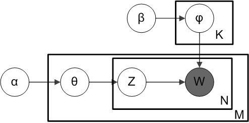
Figure 2.1: Diagram of LDA generative process

2.2 Opinion Mining (Restaurant-specific)

Given a restaurant, we propose the following analysis pipeline:
1. Extract reviewed aspects and associated text based on all reviews on the restaurant;
2. Categorize the extracted aspects into topics based on LDA results;
3. For each aspect, derive a sentiment score based on all associated text for this aspect;
4. Summarize highlights of the given restaurant based on average sentiment scores of extracted highlights.

2.2.1 Aspect Extraction

For a given text, such as “service was fast, food was pretty good and price is very affordable”, the goal is to extract aspect terms \(service\), \(food\), and \(price\), and their associated opinion \(fast\), \(pretty\ good\), and \(very\ affordable\), respectively.

Since aspect terms are primarily nouns, the candidate pool for aspects is formed by extracting all noun phrases in the given text. Noun phrases, as opposed to single words, are identified so that n-grams like “vanilla ice cream” can be extracted as a whole. At the same time, it would also make more sense to see \(vanilla\ ice\ cream\) and \(ice\ cream\) as phrases belong to the same aspect of “ice cream” to avoid redundancy. In consideration of both, we lemmatize extracted phrases to the root form (\(ice\_cream\) or \(cream\)) but also keep track of all distinct phrases under this aspect (\(vanilla\ ice\ cream\)) for potential future use.

While hundreds of aspects may be mentioned for a restaurant in its review corpus, not all of them are necessarily representative, and thus we only keep aspects mentioned by at least 10% of the reviews for this restaurant. A custom list of stopwords such as “star”, “thing”, and “customer” is also used to filter out noun chunks that are less likely to be meaningful aspects of the restaurant.

A challenge in the step of aspect extraction is parsing a sentence with multiple aspect terms into chunks corresponding to each aspect. In the example above, for the later precision of aspect-based sentiment score, I only want to attribute “fast” as opposed to other parts or the entire sentence to the specific aspect “service”. To do this, we utilize the common linguistic pattern that different aspects at the same semantic level are usually separated by a comma, “and”, or “but”: we split a mixed sentence according to these conjunctions and attribute relevant parts to concerning aspects.

2.2.2 Aspect Categorization

We experiment with two approaches for categorizing extracted aspects. Assuming some pre-fixed categories based on LDA results or conventions (we use the Annotation Guidelines for SemEval 2016 Task 5: Aspect-based Sentiment Analysis, restaurant domain), we can measure the semantic similarity between an aspect term and each of the categories and assign it to the closest category. The other approach does not make presumptions on categories, but instead try to automatically identify them through clustering.

Both approaches require some numerical representations of the aspects, and a natural choice would be using word embedding models. Word embeddings map words and phrases to vectors of real numbers using methods such as neural networks (Word2Vec) and dimensionality reduction on the word co-occurrence matrix (GloVe). For our purpose, we use a GloVe model with 300-dimensional vectors pre-trained on 42B tokens from Common Crawl. We use a pre-trained model instead of training our own on the corpus (300M tokens) in consideration of both the computation cost and the quality and size of vocabulary, and we chose the 42B-token version trained on Common Crawl since it has the largest vocab (1.9M) that could fit into the memory we have and is more suitable for our corpus comparing to the 6B-token Wikipedia in terms of the type of expression used.

For the first approach with pre-fixed categories, we use cosine similarities between each extracted aspect and the categories to determine its category; for the second approach, we use vector representations of extracted aspects to automatically identify clusters.

2.2.3 Sentiment Analysis

After parsing the review corpus for a restaurant into aspect terms and corresponding opinion sentences, we can perform sentiment analysis on the opinion sentences for each aspect term.

We recognize that both lexicon-based approach and machine learning approach can be used for this purpose. Lexicon-based methods are widely-used in the field for its intuitiveness and ease of implementation, but have limited coverage of lexical features and are not quite adaptive (manually expanding the lexicon is extremely labor-intensive and time-consuming). Machine learning methods, on the other hand, are much more flexible and often lead to better accuracy, but as with high-quality sentiment lexicons for lexicon-based methods, extensive training data are essential to the performance and validity of machine learning methods but often hard to acquire. Additionally, texts in online reviews are often short and sparse, and thus pose a challenge for ensuring the quality and quantity of input features. arse. Practically, machine learning models can also be quite expensive to implement computationally, especially when dealing with an enormous corpus. Last but not least, machine learning methods can become “black boxes” and lose interpretability.

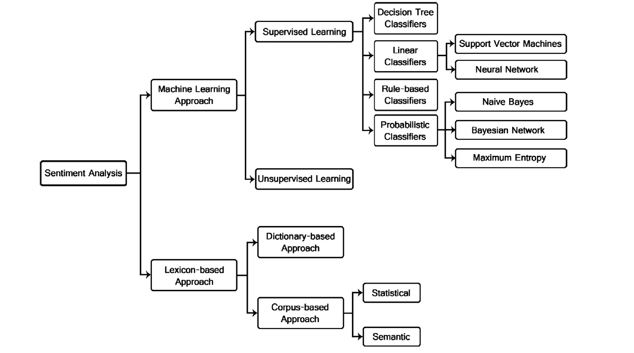
Figure 2.2: Sentiment analysis / classificaion techniques

Based on the discussion above, we decide to take a primarily lexicon-based approach (more specifically a dictionary-based approach) for the scope of this project. We experimented with two open-source implementations of refined lexicon-based sentiment analysis. One is VADER (Valence Aware Dictionary and sEntiment Reasoner), which combines a sentiment lexicon specifically attuned to social media context with grammatical and syntactical heuristics that capture intensity of sentiment, and the other is TextBlob, which uses a lexicon of adjectives (eg. good, bad, amazing, irritating etc.) that occur frequently in product reviews and takes into account semantic patterns when averaging the polarity for lexical features (eg. words). Online reviews do share many common characteristics with social media texts in terms of the distinctive way of expression and relative informality of language. Many of these characteristics, such as the prevalence of slang words, acronyms, and emoticons and the use of all caps and excessive punctuations, though commonly cleaned in the pre-processing step or simply ignored by traditional sentiment analysis tools, may contain valuable information about the polarity and intensity of sentiment. The table below shows a representative sample of challenging cases in sentiment analysis (especially in the social media/ online review context) and a comparison of results from VADER and TextBlob against the baseline of AFINN scores. As expected, VADER is quite sensitive to the intensity as well as binary polarity of sentiment, while TextBlob also has decent performance. The implementations are not without their shortcomes: VADER does seem to have a denser score distribution but at the same time also slightly dramatic changes in score in presence of emoticons and qualifications, and TextBlob tends to ignore slang words and abbreviations, but overall the two lexicon-based methods are giving reasonable results.

Table 2.1: Common challenges in sentiment analysis and comparison of performances between VADER and TextBlob against baseline results from AFINN score.
Challenge	Example text	AFINN	VADER	TextBlob
Punctuation (intensify)	Food was good!!!	0.6	0.58	1.0
Word shape (intensify)	Food was GOOD.	0.6	0.56	0.7
Emoticon	Food was good :)	0.6	0.71	0.6
Degree modifier	Food was very good.	0.6	0.49	0.9
Baseline (positive)	Food was good.	0.6	0.44	0.7
Negation	I did not dislike the food.	-0.4	0.29	0.0
Baseline (neutral)	Food was okay.	0.0	0.23	0.5
Qualification (mild negative)	Food was okay but I would not recommend it to you.	0.4	-0.30	0.5
Contraction as negation	Food was not very good.	0.6	-0.39	-0.3
Slang word	Food sux.	0.0	-0.36	0.0
Baseline (negative)	Food was bad.	-0.6	-0.54	-0.7

For each aspect, we aggregate a sentiment score using the sum of polarity scores for all review text associated with this aspect, divided by the number of reviews mentioning this aspect to account for both the volume of opinions expressed towards this aspect and the number of units (reviews) in which they were expressed.