Chapter 5 Methodology
5.1 Geographic Level
The question we would like to pose - how the distributions of toxicity that individuals experience over time are predicted by their complex, multidimensional identities - is inherently intended to use individuals as the unit of analysis. Until now environmental justice work has used census geographies or point sources as the unit of analysis.
We depend on two data sources, the disaggregated RSEI toxic release data (as compiled to contain only releases that are consistently reported between 1990 and 2010) as well as relevant demographic information from the Census.
RSEI toxicity data can be obtained at extremely fine level (the 800m by 800m grid across the United States,) but the finest grain Census data is available at is the block level, where blocks contain between 0 and a few thousand people. At such low geographic levels, cross tabulations aren’t available for demographics due to identifiability concerns. Using a low level of geography (like census blocks or block groups) is important for the environmental aspect of this analysis, since environmental hazards can be very localized, especially along neighborhood lines in urban areas.
Unfortunately, the availability of cross tabulations is equally important to the goal of this work in examining inequality of environmental burden held by minority groups in the United States. The intersection of social identities, especially those steeped in systems of oppression, is extremely important for identifying unequal burdens. For example, low income populations across the board may be more likely to experience environmental hazards, but low income minority populations may be much more likely than low income white populations to experience extreme hazard. The intersections of demographic characteristics, such as race and income or race and education are likely to be important in teasing out the true inequality burden.
We combine the computed aggregated toxicity for each block group and the demographic data. Now for each census geography, we have toxicity information as well as demographic data.
| block | concentration | area | total_pop | white | black |
|---|---|---|---|---|---|
| 010010201001 | 627.3050 | 6.520168 | 530 | 447 | 83 |
| 010010201002 | 499.6298 | 8.486690 | 1282 | 1099 | 126 |
| 010010202001 | 578.8312 | 3.137173 | 1274 | 363 | 824 |
| 010010202002 | 756.3733 | 1.962949 | 944 | 458 | 477 |
| 010010203001 | 637.7356 | 5.907125 | 2538 | 2152 | 384 |
| … | … | … | … | … | … |
We can aggregate to a national distribution of experienced toxicity by weighting each block toxicity by the number of people that experience it. This approach is restricted by Census data availability, since we can only build a distribution for each of the cross tabulations we have available. For higher levels of geography (where we might, for example, have race by income) we would be able to build national distributions for each income by race group.
In the case of the table above, to build a distribution for the white population, we would assign 447 people a toxicity of ~627, 1099 people a toxicity of ~499 and so on until we have the full distribution of toxicities experienced by the white population.
To choose the level of aggregation at which we calculate toxicity distributions, we create the overall toxicity distribution for Americans at each of the levels of geography. The process described can be executed with the data shown above, or at a cruder level of geography, such as state or region. Using block group as the smallest form of geography, and state as the largest we build toxicity distributions at each level of aggregation.
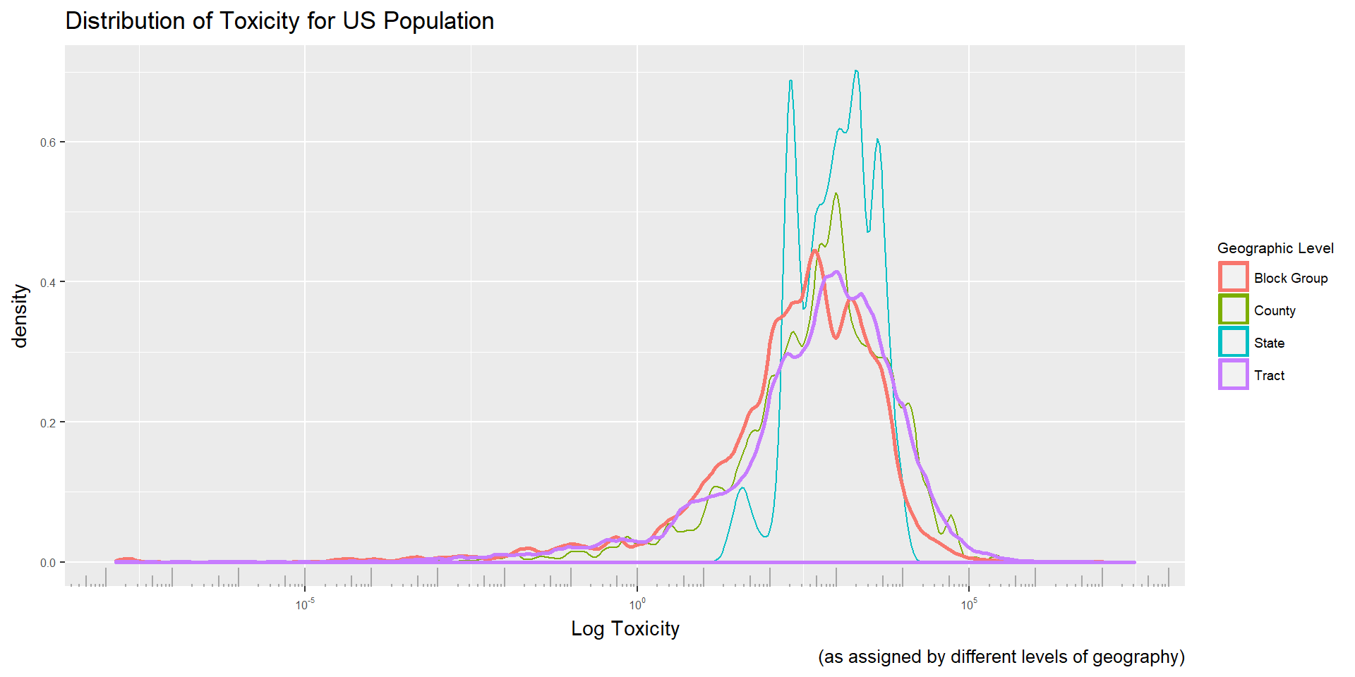
As expected, the state level assignment is a poor approximation of the lower level assignments. Given that we are assigning each individual the mean toxicity in their entire state, we are eliminating most of the variation from the data. Interestingly tract and county data seems to build a distribution quite similar to the block group level assignment. Initial results were replicated using all 3 levels of assignment, and conclusions remained the same. This may be because the block group level is aggregating a large enough group of our fine grain toxicity data that it has already lost the street block by street block variation that we had deemed so crucial, meaning aggregating several block groups gives us a conceptually equivalent ‘neighborhood’ level of aggregation.
The ecological fallacy is a constant discussion in environmental justice literature. It is speculated to be the reason for varying results, as toxicity data can be sensitive to geographic level of analysis, time of collection, and area. In this case, conclusions appear to be relatively robust to unit of assignments.
5.2 Simulation
5.2.1 Process
To examine how environmental burden changes over time for minority groups we use simulation to tease apart the forces at play in each group’s changing distributions. We expect the mean of minority distributions to reduce over time for two reasons: the toxicity distribution for the entire population is slowly shifting right and compressing as we see improvements in environmentally friendly production technology and more comprehensive environmental regulation; secondly, we hope that with Title VI protections and the work of civil rights advocates, minority communities will be better equipped to mobilize against polluters, shifting the mean of minority distribution right relative to the overall distribution.
These two explanations for decreasing toxicity can translate into two descriptors of distributional change:
distributional convergence: where inequality is reduced due to compression of the overall distribution, disproportionately improving toxicity for those at the right tail.
positional convergence: where inequality is reduced due to shifting distributions, reducing the difference between means of each distribution.
Positional convergence is of primary interest, since it would allow us to look at how much ‘true’ change there has been. By removing the distributional convergence we are able to compare the current observed reductions in inequality to what those changes would have been if minority populations had held static their position in the overall distribution.
In order to find the positional convergence of minority distributions over the period of study, we use the percentiles that minority individuals held in the overall distribution at the start of the period of study and propagate them forward to simulate what each group’s distribution would have been in later years. This simulation procedure was first discussed by Bayer, Patrick and Kerwin as a method of identifying the true gains in ‘Black-White Earning Differences’ (2016).
This simulation proceeds as follows:
Build an empirical distribution of toxicity experienced for the entire population and for each group of interest in the starting year.
Sample individuals from the empirical distributions of the groups of interest.
For each sampled toxicity value, find the percentile it holds in the empirical distribution for the entire population in the starting year.
Create an empirical distribution for the entire population in the ending year.
For each sampled percentile, find the corresponding toxicity value in the full empirical distribution of the ending year and compile results to create a simulated group of interest.
Using this method we can hold constant the place each individual (and more broadly each group) holds in the overall distribution, but follow the changes in the distribution as a whole. The collection of values simulated now represents the toxicity each individual or group would have experienced if they had held the same relative position in the overall toxicity distribution.
If there had been positional improvement for a group, we would expect the simulated distributions to paint a bleaker picture of the inequalities of environmental burden borne than the observed distribution of the ending year.
5.2.2 Accuracy
In order to estimate the standard errors of simulated estimates of the 5th, 50th and 95th percentiles, we repeatedly execute the simulation process on data for the black population in 1990. Simulating the changes of the entire black population would mean dealing with a population of around 29 million, but with a large sample we should be able to get a good estimate.
To determine how large the sample needs to be, we run the simulation 20 times for each n tested and show the mean and standard error of the estimate.
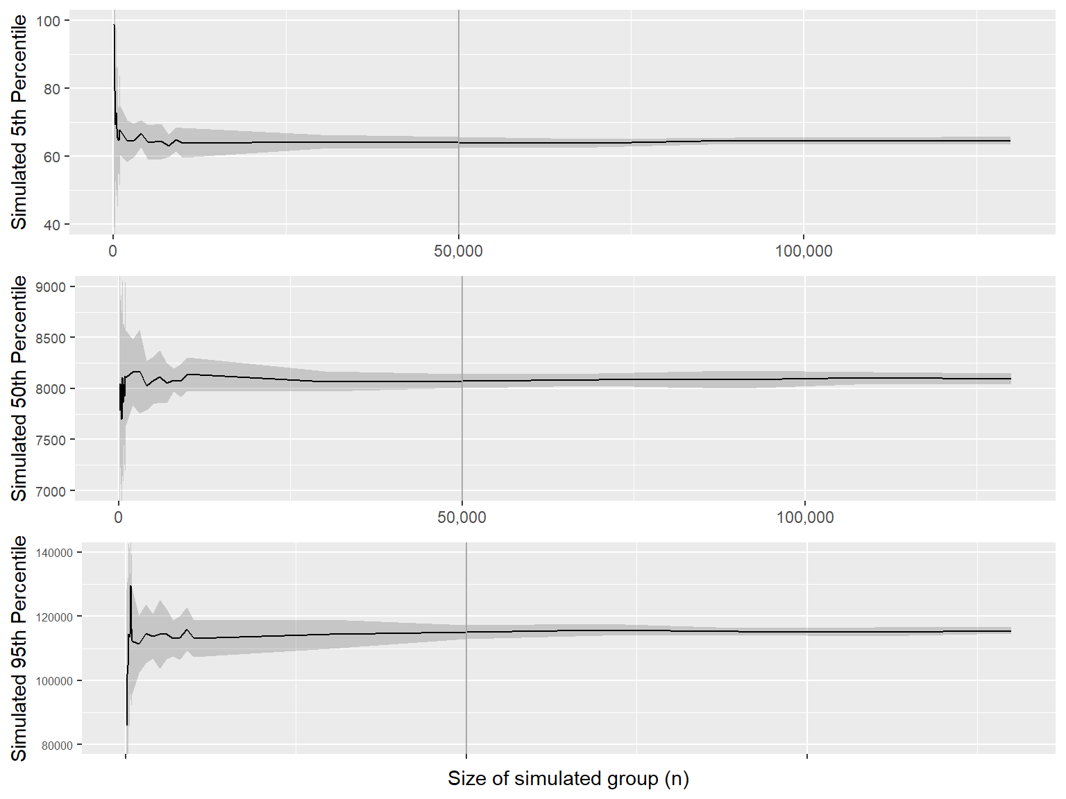
For the 5th percentile, a relatively small sample produces a fairly stable result, as standard error does not reduce substantially with n larger than 20,000. Due to the extreme right skew of the data, the 95th percentile requires a larger sample to reach a stable estimate. Still n = 50,000 is sufficient, and that size is used for all samples.