Chapter 3 Preliminary Data Investigation
3.1 Exploratory Data Analysis
3.1.1 Cleaning Predictors
sapply(argus, class) Flgs SrcAddr Sport DstAddr Dport SrcPkts DstPkts
"factor" "factor" "factor" "factor" "factor" "integer" "integer"
SrcBytes DstBytes State
"integer" "integer" "factor" argus = transform(argus,
Sport = as.factor(argus$Sport),
Dport = as.factor(argus$Dport))
argus = subset(argus, select = c("Flgs", "SrcAddr", "Sport", "DstAddr", "Dport",
"SrcPkts", "DstPkts", "SrcBytes", "DstBytes", "State"))
attach(argus)
categorical = c("Flgs", "SrcAddr", "Sport", "DstAddr", "Dport", "State")
continuous = c("SrcPkts", "DstPkts", "SrcBytes", "DstBytes")This code casts the features to their corresponding class classifications (numeric and factor), and removes Proto, StartTime, and Diretion from the dataset.
3.1.2 Categorical Features: Unique Categories and Counts
sapply(argus, function(x) length(unique(x))) Flgs SrcAddr Sport DstAddr Dport SrcPkts DstPkts SrcBytes
70 65113 64486 41903 17537 2790 3633 44075
DstBytes State
64549 6 #function that returns elements of the feature and their counts in descending order
element_counts = function(x) {
dt = data.table(x)[, .N, keyby = x]
dt[order(dt$N, decreasing = TRUE),]
}
element_counts(Sport) x N
1: 33461 35683
2: 4263 8541
3: 80 8346
4: 4165 4988
5: 48468 3023
---
64482: 57904 1
64483: 58242 1
64484: 59051 1
64485: 59315 1
64486: 60116 1element_counts(Dport) x N
1: 23 235616
2: 80 204128
3: 443 137360
4: 32819 102166
5: 25 53167
---
17533: 65515 1
17534: 65528 1
17535: 65529 1
17536: 65532 1
17537: 65533 1element_counts(SrcAddr) x N
1: 197.0.31.231 35440
2: 1.0.11.96 8717
3: 100.0.7.149 8526
4: 197.0.9.1 5536
5: 1.0.85.103 4976
---
65109: 197.0.55.5 1
65110: 197.0.55.6 1
65111: 197.0.55.7 1
65112: 197.0.55.8 1
65113: 197.0.55.9 1element_counts(DstAddr) x N
1: 100.0.1.9 64508
2: 100.0.1.2 62681
3: 100.0.1.28 25780
4: 100.0.1.55 25641
5: 100.0.18.93 20766
---
41899: 100.0.6.179 1
41900: 100.0.7.173 1
41901: 100.0.77.113 1
41902: 100.0.77.147 1
41903: 100.0.88.111 1element_counts(State) x N
1: REQ 571899
2: FIN 307337
3: RST 135280
4: CON 17146
5: ACC 16815
6: CLO 983.1.3 Continuous Features: Distributions and Relationships
par(mfrow=c(2,2))
hist(SrcBytes); hist(SrcPkts); hist(DstBytes); hist(DstPkts) #clearly some very large values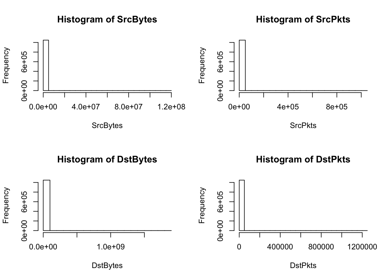
largest_n = function(x, n){
  head(sort(x, decreasing=TRUE), n)
}
largest_n(SrcBytes, 10)
[1] 118257047 116615879 112673526 108933442 105793666 73376579 72839115
[8] 70001807 56206409 55359912largest_n(SrcPkts, 10) [1] 1008233 1000971 771590 492361 458603 437296 408530 407973
[9] 371976 371251largest_n(DstBytes, 10) [1] 1850817751 1713055847 1690162763 1524781880 1491609296 1340922625
[7] 1304668214 1206594243 1163954979 1145323438largest_n(DstPkts, 10) [1] 1239611 1223485 1219276 1004471 982931 942827 883354 795120
[9] 766776 754831The histograms and the largest 10 values in each of the continuous variables show that there are a relatively few amount of large observations skewing the distributions. This explains the model summary containing means much larger than their medians. It’s not possible to remove the large values as outliers because they may be scanner observations to detect. Also there is a high frequency (up to the first quartile) of destination bytes and packets that equal 0.
We will now try to investigate whether the largest continuous predictor values correspond to any particular addresses or ports.
max.SrcBytes = argus[with(argus,order(-SrcBytes)),][1:20,]
max.SrcPkts = argus[with(argus,order(-SrcPkts)),][1:20,]
max.DstBytes = argus[with(argus,order(-DstBytes)),][1:20,]
max.DstPkts = argus[with(argus,order(-DstPkts)),][1:20,]
head(max.SrcBytes)
Flgs SrcAddr Sport DstAddr Dport SrcPkts DstPkts
282859 * s 1.0.12.1 18086 100.0.1.8 31743 208339 104886
282841 * s 1.0.12.1 18086 100.0.1.8 31743 204912 99688
282832 * s 1.0.12.1 18086 100.0.1.8 31743 198007 94621
282853 * s 1.0.12.1 18086 100.0.1.8 31743 191443 95892
282823 * s 1.0.12.1 18086 100.0.1.8 31743 186228 84342
724162 * * 100.0.4.9 37901 100.0.2.67 22 1008233 1239611
SrcBytes DstBytes State
282859 118257047 7514403 CON
282841 116615879 7146182 CON
282832 112673526 6801146 CON
282853 108933442 6857053 CON
282823 105793666 6048529 CON
724162 73376579 1713055847 CONhead(max.DstBytes) Flgs SrcAddr Sport DstAddr Dport SrcPkts DstPkts
2162 * d 197.0.1.1 62030 100.0.1.1 80 371251 1219276
724162 * * 100.0.4.9 37901 100.0.2.67 22 1008233 1239611
724106 * * 100.0.4.9 37901 100.0.2.67 22 1000971 1223485
2212 * d 197.0.1.1 62034 100.0.1.1 80 280593 1004471
78245 * d 1.0.2.1 11210 100.0.1.2 80 158194 982931
2185 * d 197.0.1.1 62033 100.0.1.1 80 268402 883354
SrcBytes DstBytes State
2162 26430322 1850817751 CON
724162 73376579 1713055847 CON
724106 72839115 1690162763 CON
2212 20037592 1524781880 FIN
78245 11294111 1491609296 CON
2185 19137354 1340922625 FINSource Addresses tend to be repetitive for the largest max bytes/packets, while ports vary. The top 10 largest DstBytes all correspond to SrcAddr 197.0.1.1 and DstAddr 100.0.1.1. Also both max Src and Dst rows correspond to the “* s”" flag. The largest sizes of DstBytes tend to go to Dport 80, which is the port that expects to receive from a web client (http), while the largest SrcBytes go to 31743. The next section implements a systematic way for investigating the relationship between addresses and ports because simply looking at the max rows is difficult.
3.1.4 Correlation Between Features
cor(SrcBytes, SrcPkts)[1] 0.5732968cor(DstBytes, DstPkts)[1] 0.996775cor(SrcBytes, DstBytes)[1] 0.3331221cor(SrcPkts, DstPkts)[1] 0.8448269The plots of the predictors suggest strong linear trends between the predictors, which makes intuitive sense given the domain matter. Further investigations show that DstPkts has a correlation of ~1 with DstBytes and ~0.85 with SrcPkts.
cor(DstBytes, DstPkts, method = "kendall")
cor(SrcPkts, DstPkts, method = "kendall")
cor(DstBytes, DstPkts, method = "spearman")
cor(SrcPkts, DstPkts, method = "spearman")
Because the original correlation tests relied on the Pearson method, which is susceptible to bias from large values, further tests investigate the relationship between DstPkts and the other features. While the correlation is still high for Kendall-Tau and Spearman’s correlation coefficients, it is less cause for concern when compared to the skewed response from the Pearson method.
3.2 Transformations on the Data
3.2.1 Removing Quantiles
To get a better sense of the unskewed distribution, the below plots visualize the continuous features with the largest and smallest 10% of observations removed. The removed values will be readded to the dataset when investigating for anomalies.
remove_quantiles = function(v, lowerbound, upperbound){
  return (v[quantile(v,lowerbound) >= v & v <= quantile(v,upperbound)])
}
SrcBytes.abrev = remove_quantiles(SrcBytes,0.10,0.9)
SrcPkts.abrev = remove_quantiles(SrcPkts,0.10,0.9)
DstBytes.abrev = remove_quantiles(DstBytes,0.10,0.9)
DstPkts.abrev = remove_quantiles(DstPkts,0.10,0.9)
par(mfrow=c(2,2))
hist(SrcBytes.abrev); hist(SrcPkts.abrev); hist(DstBytes.abrev); hist(DstPkts.abrev)
The continuous features are still unevenly distributed even with the 20% most extreme values removed.
3.2.2 Log Transformation
par(mfrow=c(2,2))
hist(log(SrcBytes)); hist(log(SrcPkts)); hist(log(DstBytes)); hist(log(DstPkts))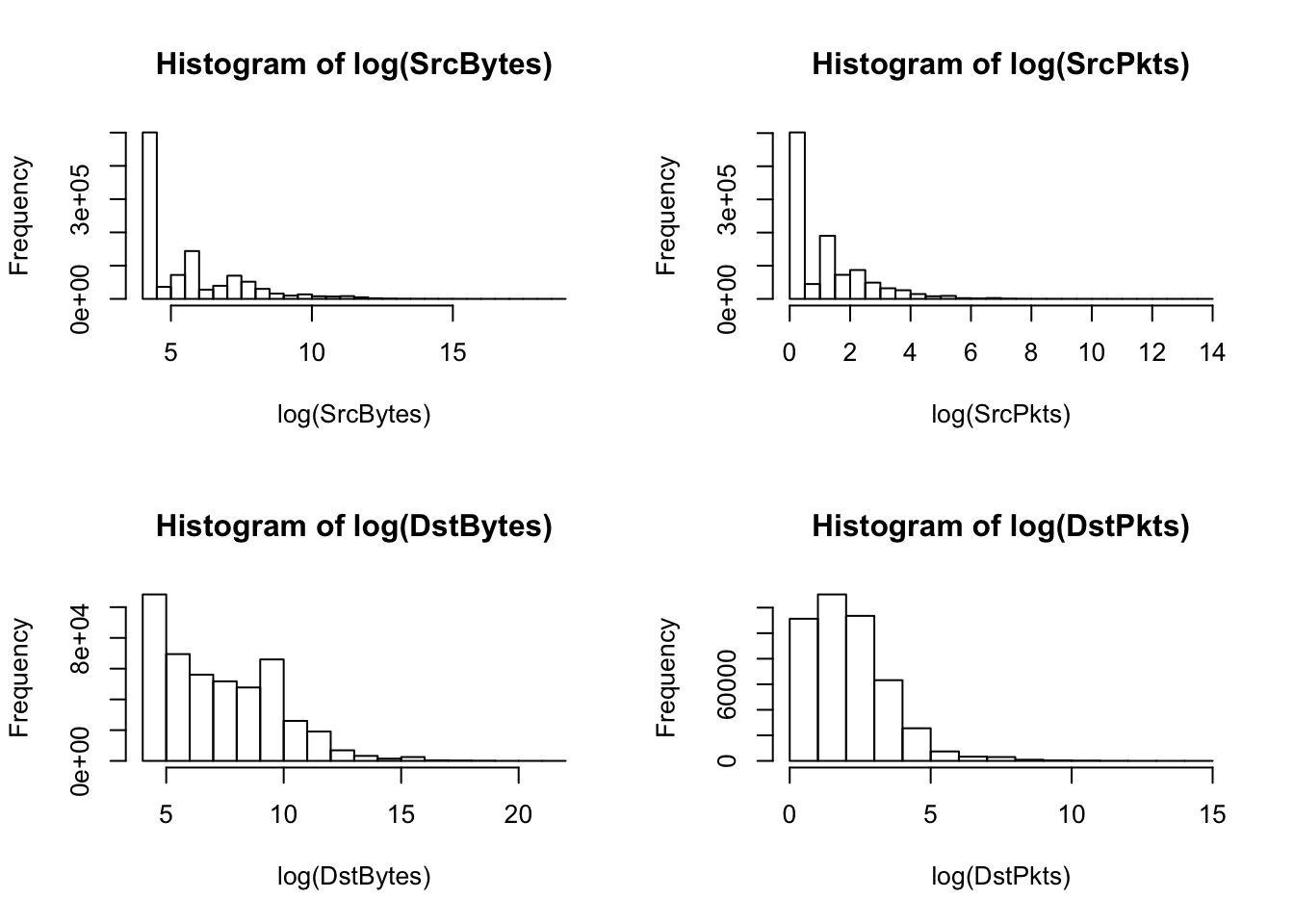
plot(log(SrcPkts), log(SrcBytes)); plot(log(DstPkts), log(DstBytes))
plot(log(SrcBytes), log(DstBytes)); plot(log(SrcPkts), log(DstPkts))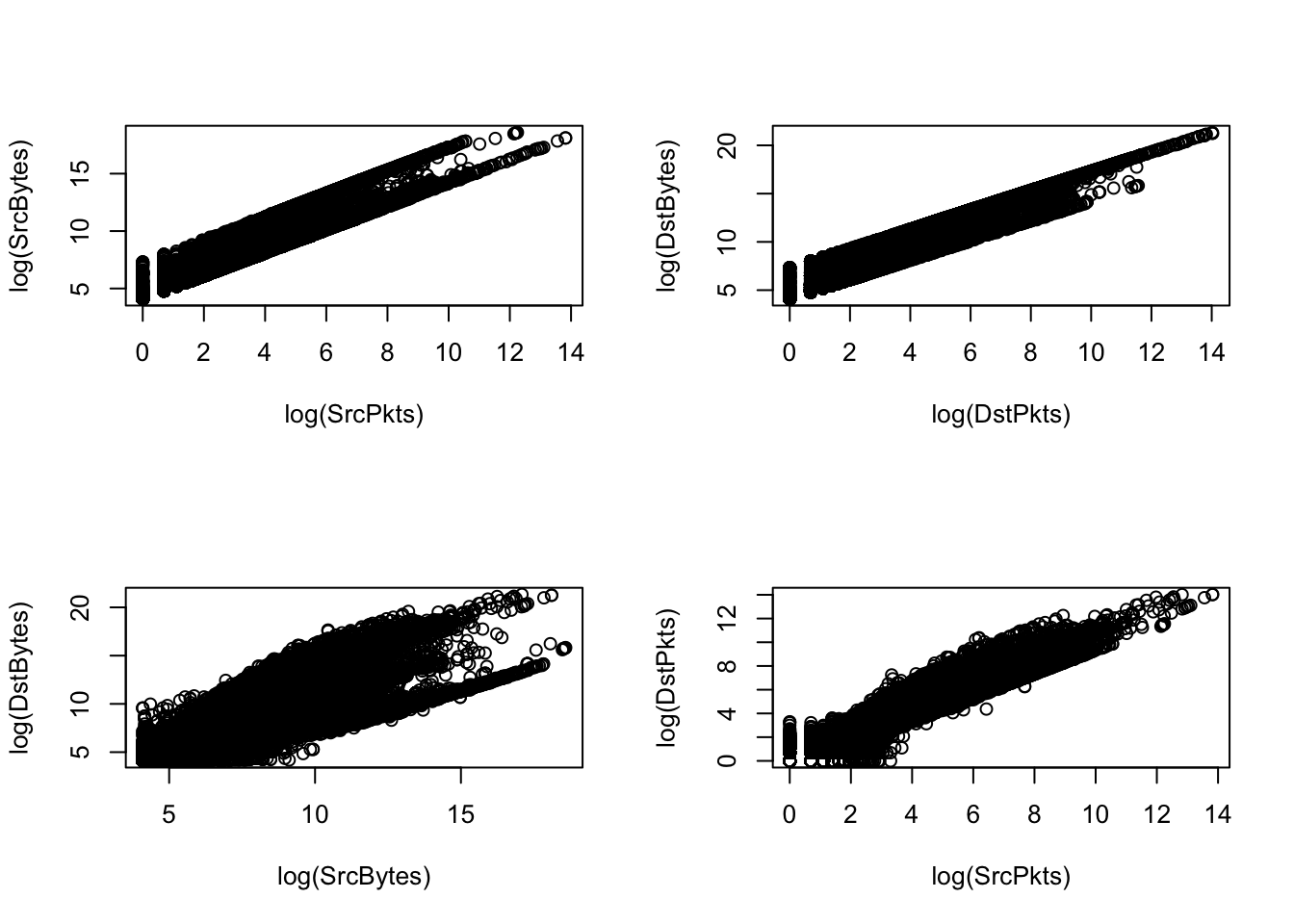
A log transformation for each of the continuous features outputs right-skewed histograms. Skewed features may affect the results of a kernel pca, so we consider other approaches for transformations.
3.2.3 Normal Scores Transformation
nscore = function(x) {
   # Takes a vector of values x and calculates their normal scores. Returns
   # a list with the scores and an ordered table of original values and
   # scores, which is useful as a back-transform table. See backtr().
   nscore = qqnorm(x, plot.it = FALSE)$x  # normal score
   trn.table = data.frame(x=sort(x),nscore=sort(nscore))
   return (list(nscore=nscore, trn.table=trn.table))
}

backtr = function(scores, nscore, tails='none', draw=TRUE) {
   # Given a vector of normal scores and a normal score object
   # (from nscore), the function returns a vector of back-transformed
   # values
   # 'none' : No extrapolation; more extreme score values will revert
   # to the original min and max values.
   # 'equal' : Calculate magnitude in std deviations of the scores about
   # initial data mean. Extrapolation is linear to these deviations.
   # will be based upon deviations from the mean of the original
   # hard data - possibly quite dangerous!
   # 'separate' :  This calculates a separate sd for values
   # above and below the mean.
   if(tails=='separate') {
      mean.x <- mean(nscore$trn.table$x)
      small.x <- nscore$trn.table$x < mean.x
      large.x <- nscore$trn.table$x > mean.x
      small.sd <- sqrt(sum((nscore$trn.table$x[small.x]-mean.x)^2)/
                       (length(nscore$trn.table$x[small.x])-1))
      large.sd <- sqrt(sum((nscore$trn.table$x[large.x]-mean.x)^2)/
                       (length(nscore$trn.table$x[large.x])-1))
      min.x <- mean(nscore$trn.table$x) + (min(scores) * small.sd)
      max.x <- mean(nscore$trn.table$x) + (max(scores) * large.sd)
      # check to see if these values are LESS extreme than the
      # initial data - if so, use the initial data.
      #print(paste('lg.sd is:',large.sd,'max.x is:',max.x,'max nsc.x
      #     is:',max(nscore$trn.table$x)))
      if(min.x > min(nscore$trn.table$x)) {min.x <- min(nscore$trn.table$x)}
      if(max.x < max(nscore$trn.table$x)) {max.x <- max(nscore$trn.table$x)}
   }
   if(tails=='equal') { # assumes symmetric distribution around the mean
      mean.x <- mean(nscore$trn.table$x)
      sd.x <- sd(nscore$trn.table$x)
      min.x <- mean(nscore$trn.table$x) + (min(scores) * sd.x)
      max.x <- mean(nscore$trn.table$x) + (max(scores) * sd.x)
      # check to see if these values are LESS extreme than the
      # initial data - if so, use the initial data.
      if(min.x > min(nscore$trn.table$x)) {min.x <- min(nscore$trn.table$x)}
      if(max.x < max(nscore$trn.table$x)) {max.x <- max(nscore$trn.table$x)}
   }
   if(tails=='none') {   # No extrapolation
      min.x <- min(nscore$trn.table$x)
      max.x <- max(nscore$trn.table$x)
   }
   min.sc <- min(scores)
   max.sc <- max(scores)
   x <- c(min.x, nscore$trn.table$x, max.x)
   nsc <- c(min.sc, nscore$trn.table$nscore, max.sc)

   if(draw) {plot(nsc,x, main='Transform Function')}
   back.xf <- approxfun(nsc,x) # Develop the back transform function
   val <- back.xf(scores)
   return(val)
}

SrcBytes_norm = nscore(SrcBytes)$nscore
SrcBytes_table = nscore(SrcBytes)$trn.table

SrcPkts_norm = nscore(SrcPkts)$nscore
SrcPkts_table = nscore(SrcPkts)$trn.table

DstBytes_norm = nscore(DstBytes)$nscore
DstBytes_table = nscore(DstBytes)$trn.table

DstPkts_norm = nscore(DstPkts)$nscore
DstPkts_table = nscore(DstPkts)$trn.table
par(mfrow=c(2,2))
hist(SrcBytes_norm); hist(SrcPkts_norm); hist(DstBytes_norm); hist(DstPkts_norm)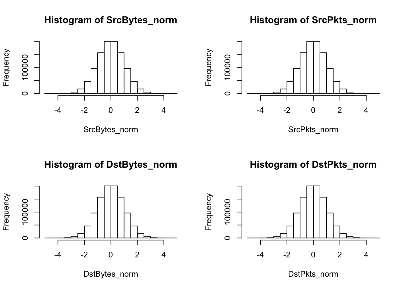
Finally, a normal scores transformation is applied to the dataset. The normal scores transformation reassigns each feature value so that it appears the overall data for that feature had arisen or been observed from a standard normal distribution. This transformation solves the issue of skewness-each value’s histogram will now follow a standard gaussian density plot-, but it may cause issues with other analysis methods, particularly methods that are susceptible to ties in data.